h1=1           #Handling time of prey type 1 (s)
h2=60          #Handling time of prey type 2 (s)
a2=0.05 #abundance of prey type 2 (ind/s)2 Economic models of behavior: do animals optimize?
🚧 This chapter is under construction. Content may change.
Animals have to make decisions all the time: where and when to move, when and what to eat, whom to mate, etc. How do animals make those decisions? One approach to study this question is to assume that animals take decisions that maximize their fitness. This approach is rooted in the idea that natural selection, under certain conditions, maximize the average fitness of individuals in a population. It underpins many of the studies in behavioral ecology, and lead to the development during the 1970’s and 1980’s.of a sub-field dedicated to the study of foraging decisions, known as optimal foraging (see for instance Pyke 1984). The idea of optimal foraging is to develop economic models of foraging behavior, assessing the costs and benefits of different actions, and identifying in any particular circumstance the action that maximizes benefits and minimizes costs. This is, animals are seen as optimizer of decision-making. Here we consider models for two “idealized” types of foragers: searching predator and sit-and-wait predators.
2.1 Searching predator
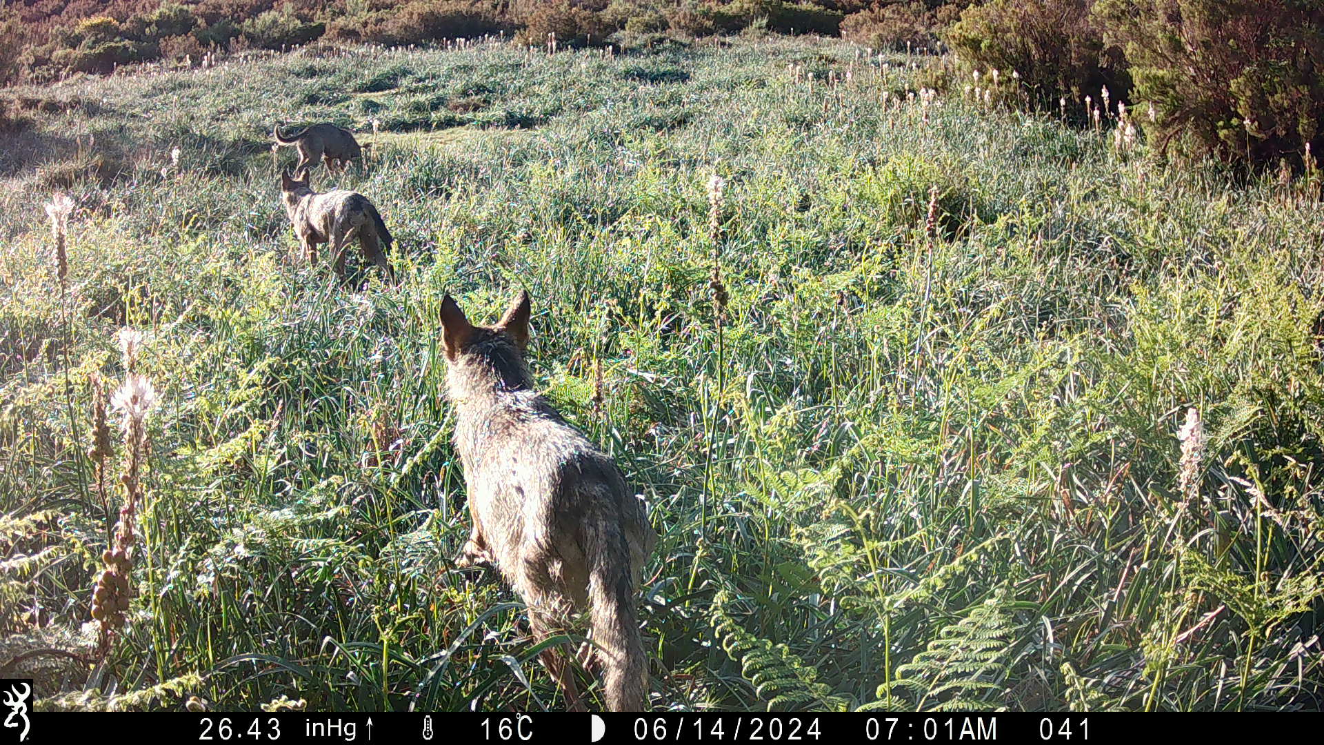
The searching predator is typified as an animal that actively searchs for food. For instance, wolfs roam the landscape constantly searching for their prey (Figure 2.1). The question is then, any time that a forager comes across a prey whether to spend the time catching and eating it, or continuing to search for another prey, for instance a larger or easier prey item. Joan Roughgarden also liked this type of foraging to the sushi-bar problem where dishes are coming one after the other on a moving tray, and a person needs to decide whether to pick a given dish. This decision is particularly akin to the searching predator situation when one assumes that a person can have only one dish at a time in her or his table, We consider two types of searching predators: time minimizers and energy maximizers.
2.1.1 Time minimizer
Many searching predators are themselves preys to other animals. For instance shrews search for insects to eat, but can be themselves eaten by carnivores or owls. Therefore a reasonable assumption is that they are making foraging decisions that minimize the time foraging. Let’s assume there are two types of prey items, type 1 and 2. These two preys occur at different abundances in the environment, let’s name them \(a_1\) and \(a_2\). These abundances can be measured as encounter rates from the predator perspective, this is the number of prey items found per unit time. The two types of prey also have different handling times, this is the amount of time required to chase and process the prey, \(h_1\) and \(h_2\) . We also convention to call the type 1 prey the prey with the lowest handling time, i.e. \(h_1<h_2\),
A searching predator can adopt one of the following three strategies:
Strategy 1: to consume only prey items of type 1
Strategy 2: to consumer only prey items of type 2
Strategy 1&2: to consumer both types of prey
In order to find out which strategy should be adopted by the forager, one needs to calculate the average spent per food item in each of the strategies. For Strategy 1 the average time per item, \(T_1\) is the sum of the amount of time the predator needs to encounter a prey with the amount of time that it takes to process that prey. As the abundance is measured in encounter rates, i.e. prey items per unit time, the inverse of that is the waiting time for a prey. Therefore we have for Strategy 1,
\[T_1=1/a_1+h_1 \tag{2.1}\]
Similarly, for Strategy 2, the average time per item \(T_2\) is given by
\[T_2=1/a_2+h_2. \tag{2.2}\]
A more interesting case is Strategy 3. Here the waiting time is the inverse of the sum of the abundances of both times of prey, while the handling time is average of the handling times of both ypes of prey weighted by their relative abundance,
\[ T_{3}=\frac{1}{a_1+a_2}+\frac{a_1 h_1+a_2 h_2}{a_1+a_2} \tag{2.3}\]
We can now define the problem that the forager has to solve as to find the strategy \(i\) that minimizes \(T_i\):
\[ min(T_i) \quad \text{for} \quad i=1, 2, 3 \]
It is easy to demonstrate that Strategy 2 is always worse than Strategy 3, independently of the abundances of the two types of prey. This happens because Strategy 3 always implies a longer waiting time than the two other specialized strategies (i.e. one has to wait less time to find any item of an prey than items of a given prey time, \(1/(a_1+a_2)<1/a_2\)) and the handling time of strategy 3 can never be higher than the handling time of strategy 2 (it’s always a value betwen \(h_1\) and \(h_2\)). So we can exclude Strategy 2 from our analysis. The choice is then between Strategy 1, just taking items of the preferred prey item, and 3, taking items of both types of prey. Let’s assess this two strategies with a little bit of help from R. We start by assuming that the handling time of prey type 1 is 1 second while prey type 2 takes 60 seconds. Let’s also assume that the abundance of prey type 2 is 0.05 individuals per second, i.e. one individuals needs to wait in average 20 seconds to find prey type 2.
Let’s now plot the time per item of each of the strategies as a function of the abundance of the preferred prey.
a1<-seq(0.005,0.1,0.001)   #abundance of prey time 1 (ind/s)
t1=1/a1+h1                 #time per item of Strategy 1 (s)
t3=1/(a1+a2)+h1*a1/(a1+a2)+h2*a2/(a1+a2) #time per item of Strategy 2 (s)
plot(a1,t1, type="l", col="blue")
lines(a1,t3, type="l", col="red")
legend("topright",
       legend = c("Strategy 1", "Strategy 3"),  # Labels
       col = c("red", "blue"),             # Line colors
       lwd = 2,                            # Line width
lty = 1) 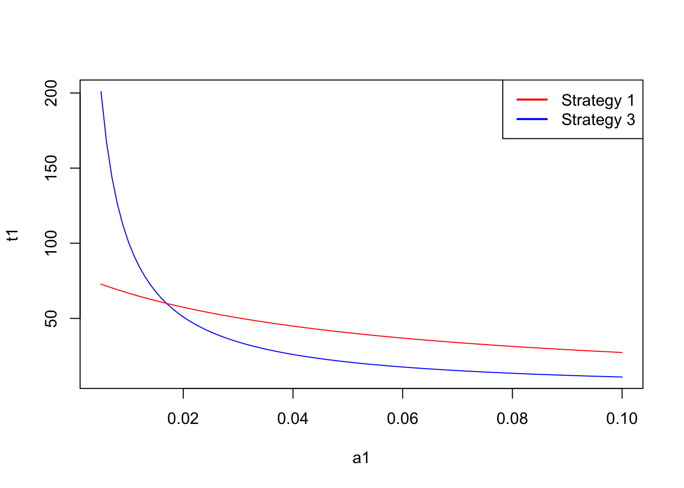
There is a critical threshold of the abundance of prey type 1 above which strategy 1 is preferrable, while below that threshold strategy 3 is the best strategy. Interestingly this threshold does not depend on the abundance of the less preferable prey. For instance, if we assume a low abundance of prey time 2 at 0.01, the resulting plot is:
a2 = 0.01
t1=1/a1+h1                 #time per item of Strategy 1 (s)
t3=1/(a1+a2)+h1*a1/(a1+a2)+h2*a2/(a1+a2) #time per item of Strategy 2 (s)
plot(a1,t1, type="l", col="blue")
lines(a1,t3, type="l", col="red")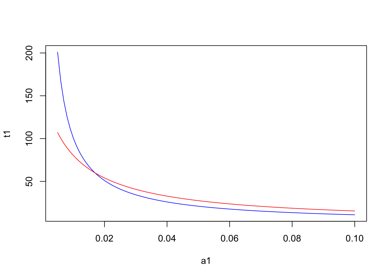
To determine this critical threshold one can compare the two vectors, T1 and T3, and find the first position at which T1 becomes smaller than T3,
pos=which(t1<t3)[1]
a1[pos]
[1] 0.017So the critical threshold for these handling times occurs when \(a_1=0.017\) individuals per second.
2.1.2 Energy per time maximizer
Perhaps more often, animals try to maximize their energy yield (benefits) while minimizing the time foraging (costs). Or in another way of looking at it, they try to maximize their energy yield per unit time. We already know the time per item associated to each of the three strategies of the searching predator. We now need to caiculate the average energy yield per item. Consider now that the energy content of the prey items are \(e_1\) and \(e_2\) for prey of type 1 and 2, respectively. We define prey 1 as the preferred type of prey, so we assume that the ratio of the energic content (measured for instance in calories) to the handling time is higher for type 1 prey, i.e. \(e_1/h_1>e_2/h_2\). Now we calculate the energy yield per item for each strategy. We start with the energy content of the prey, but need to subtract the energy spent while waiting the prey and the energy spent chasing and processing the prey,
\[ E_1=e_1-ew*tw_1-eh*h_1 \tag{2.4}\]
where \(ew\) and \(eh\) are the energy spent per unit time while waiting for the prey and the energy spent per unit time while handling, respectively. They can both be measured for instance in cal/s. We already know from the time minimizer that the waiting time for the prey is the inverse of the abundance, \(tw_1=1/a_1\). Therefore substituting in Equation 2.4 we have
\[ E_1=e_1-\frac{ew}{a_1}-eh*h_1. \tag{2.5}\]
A similar expression can be written for Strategy 2, replacing 1 with 2 in Equation 2.4.
\[ E_2=e_2-\frac{ew}{a_2}-eh*h_2. \tag{2.6}\]
More interesting is to derive the expression for Strategy 3, where the foragers takes both types of prey. The energy content of the prey is the average of the energetic contents of each prey type, weighted by their abundances, \((e_1*a_1+e_2*a_2)/(a_1+a_2)\). The waiting time is the inverse of the sums of the abundances of preys of both types, as in Equation 2.3. The handling time is the average of the handling times of each prey type, weighted by their abundances. So we have,
\[ E_3=\frac{e_1*a_1+e_2*a_2}{a_1+a_2}-\frac{ew}{a_1+a_2}-eh\frac{h_1*a_1+h_2*a_2}{a_1+a_2}. \tag{2.7}\]
Finally we can calculate the energy per unit time for each strategy by dividing Equation 2.5 by Equation 2.1 for Strategy 1, dividing Equation 2.6 by Equation 2.2 for Strategy 2, and dividing Equation 2.7 by Equation 2.3 for strategy 3,
\[ ET_i=\frac{E_i}{T_i} \]
Similarly to the time minimizer, it’s possible to show mathematically that strategy 2 is never an optimal strategy. So the interesting comparison is again between strategy 1 and strategy 3. Let’s use R to plot the energy per time yield for both strategies. We start by setting the parameter values of our model with some realistic numbers.
e1<-10                       #Caloric content of prey 1
e2<-100                      #Caloric content of prey 2
h1<-1                        #Handling time of prey 1
h2<-60                       #Handling time of prey 2
ew<-1                        #Energy spend per unit time while waiting (cal/s)
eh<-1                        #energy spend per unit time handling the prey (cal/s)
We will examine the energy yields for strategy 1 and strategy 3 for a fixed abundance of prey type 2 and a sequence of abundances of prey type 1 from 0.005 individuals per second to 0.5 individuals per second
a1<- seq(0.005,0.5,0.001)    #Sequence of abundances of prey 1
a2<-0.05
With the parameter and abundance values defined, we can calculate \(E_1\), \(E_3\), \(T_1\), \(T_3\), and then \(ET_1\) and \(ET_3\) based on the equations above, resulting in vectors for these variables with each entry in the vector corresponding to an abundance value in the vector of abundances a1.
E1 = e1 -(eh*h1) - ew/a1    #energy per item of Strategy 1 (s)
E3 = (e1*a1+e2*a2)/(a1+a2)-
     eh*(h1*a1+h2*a2)/(a1+a2)-ew/(a1+a2) #energy per item of Strategy 3 (s)

T1=1/a1+h1                 #time per item of Strategy 1 (s)
T3=1/(a1+a2)+h1*a1/(a1+a2)+h2*a2/(a1+a2) #time per item of Strategy 3 (s)

ET1 = E1/T1 #energy per time of strategy 1
ET3 = E3/T3 #energy per time of strategy 3
Next we plot the energy yields against the values of abundance of prey of type 1, and add a nice legend:
plot(a1,ET1,type="l",xlab="Abundance of prey 1", ylab="Energy per time", col="blue")
lines(a1,ET3,type="l",col="red")
legend("topright",
       legend = c("Strategy 1", "Strategy 3"),  # Labels
       col = c("red", "blue"),             # Line colors
       lwd = 2,                            # Line width
lty = 1) 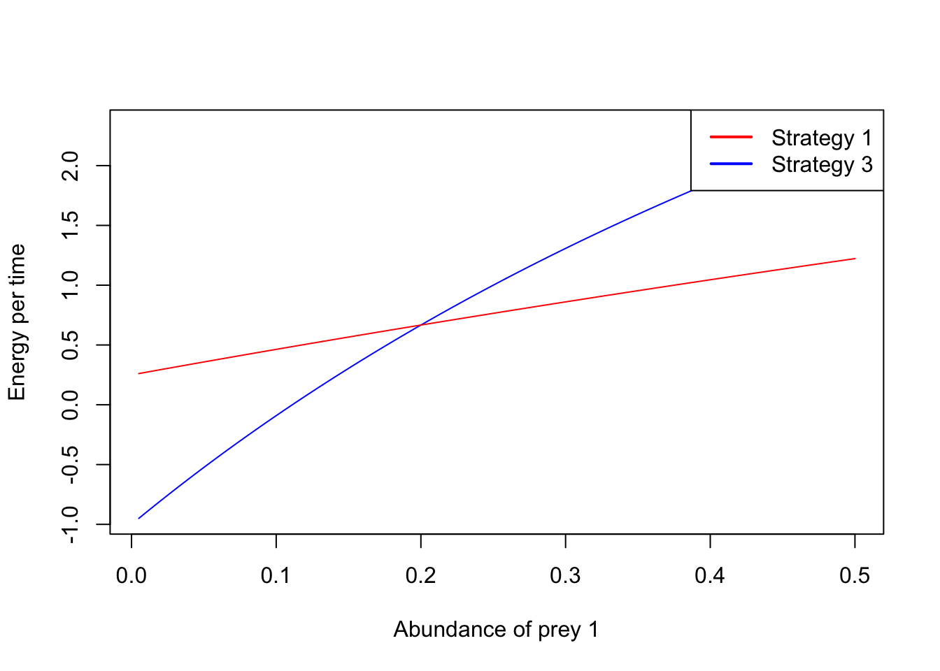
Similarly to the the time minimizer, for the energy maximizer there is also a critical threshold of the abundance of prey type 1 above which strategy 1 is preferrable, while below that threshold strategy 3 is the best strategy.
2.2 Sit-and-wait predator
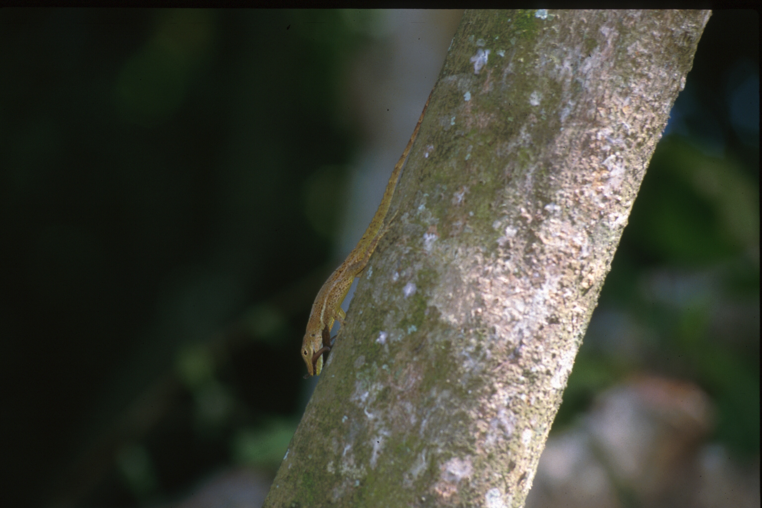
In contrast to the searching predator, the sit-and-wait predator forages by patiently ambushing its prey. For instance, the lizard Anolis gingivinus (Figure 2.2) waits in a perch, often a tree trunk, for a prey to come into its reach, sprinting then down the trunk or into the ground to capture its prey, returning then to its perch again. So here the decision that the predator has to take after seeing the prey is whether it should run an capture the prey or if it should ignore it.
We will build on the model we developed for the energy per time maximizer searching predator to develop a model for the decisions of the sit-and-wait predator. The energy per prey item consumed is,
\[ E=e-ep t_p-e_w t_w \tag{2.8}\]
where \(e_p\) is the energy per unit time while pursuing the prey, \(t_p\) is the average time it takes to sprint to the prey and come back to the perch, \(e_w\) is the energy per unit time while waiting for the prey, and \(t_w\) is the average time it takes to wait for a prey item to show up within the home-range or territory of the predator. We will use these two terms interchangeably, although they are sometimes used in the literature differently.
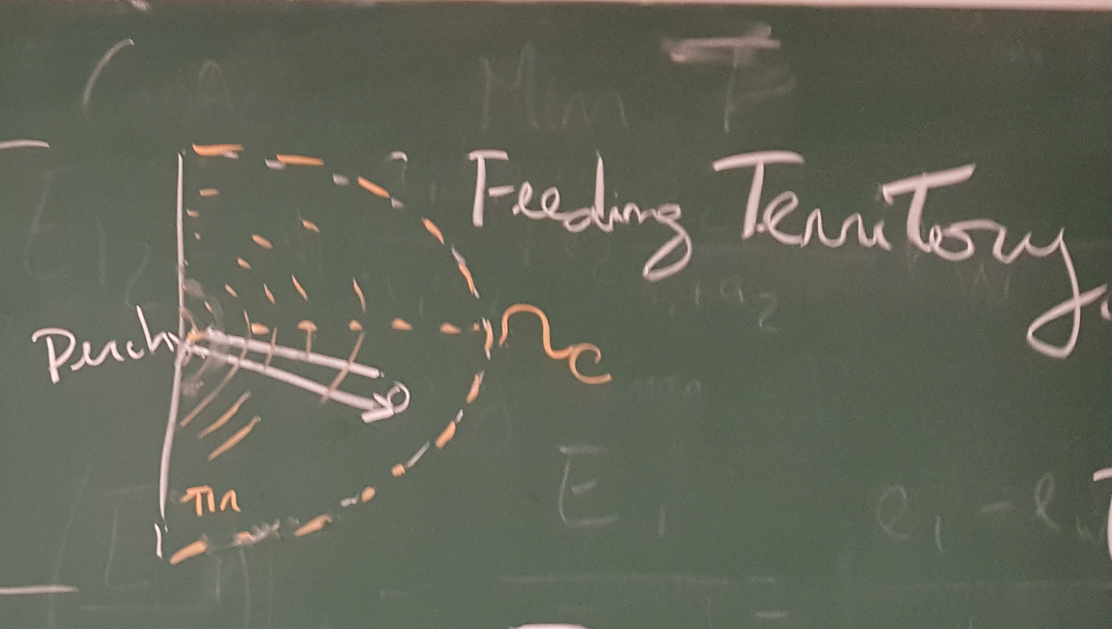
Let’s consider that the home-range of the lizard is shaped as a semi-circle centered in the perch. This is the lizard has a viewing angle of \(180\deg\) from its perch (Figure 2.3). Then the total abundance of the the prey in the territory is the integral of the prey point density over the territory. So, using polar coordinates for the integral this can be written as,
\[ A=\int_{0}^{r_c}a \pi r dr \]
The waiting time is just the inverse of the total abundance.
\[t_w=1/A=\frac{1}{\int_{0}^{r_c}a \pi r dr}\]
The average pursuit time is a bit more complicated. For a prey landing at distance \(r\) from the predator, the pursuit time is the time the lizards needs to run to that location and back. This is can be calculated by dividing the double of the distance by the speed of the lizard, \(2r/v\). We have now to average these sprint times over the range of possibile distance that the lizard can run, from 0 to the radius of its territory \(r_c\), weighted by the probability of a prey appearing at each distance. The probability of a prey appearing at distance \(r\) is the length of the semi-circle with radius \(r\) multiplied by the point density of prey divided by the total density of prey in the territory of the lizard, \(a \pi r / A\). So we now need to calculate the integral of the sprint times at each distance times the probability of running to a prey at that distance over the range of possible radius values,
\[ t_p=\int_{0}^{r_c} \frac{2r}{v} \frac{a \pi r}{A} \ dr \]
The average time per prey item consumed is simply the sum of the average pursuit time, \(t_p\), and the average waiting time \(t_w\),
\[ T=t_p+t_w \tag{2.9}\]
Therefore the energy per time that the optimal sit-and-wait predator wants to maximize is obtained by dividing Equation 2.8 by Equation 2.9,
\[ ET(r_c)=\frac{e-e_p t_p(r_c)-e_w t_w(r_c)}{t_p(r_c)+t_w(r_c)} \]
where we highlighted that the wating time and the pursuit time are functions of the territory size or cut-off radius \(r_c\).
The optimal decision is to find the cut-off radius \(r_c\) that maximizes the energy per time,
\[ \max_{r_c}(ET) \]
Let’s plot the energy per time as a function of the territory size,
ew<-0.1                  #Energy per unit of time of waiting
ep<-1                    #Energy per unit of time of pursuing the prey
v<-0.5                   #Velocity of the predator in chase
a<-0.005                 #Abundance of prey
e<-10                    #Energy value of the prey

rc<-seq(0.001,4,0.001)   #Radius of the hunting ground

tw <- 1/(a*pi*((rc^2)/2))   #Waiting time
tp<-4/3*rc/v                #Pursuing time
ti<-tw+tp                   #Time per item
ei<-e-ew*tw-ep*tp           #Energy per item
et<-ei/ti                   #Energy per unit of time

et <-function()
{
  (e-ew*(1/(a*pi*((rc^2)/2)))-ep*(4/3*rc/v))/(1/(a*pi*((rc^2)/2))+4/3*rc/v)
}

plot(rc,et(),type="l",
     xlab="Radius of the territory",
     ylab="Energy per unit of time (cal/sec) ")
 abline(0,0)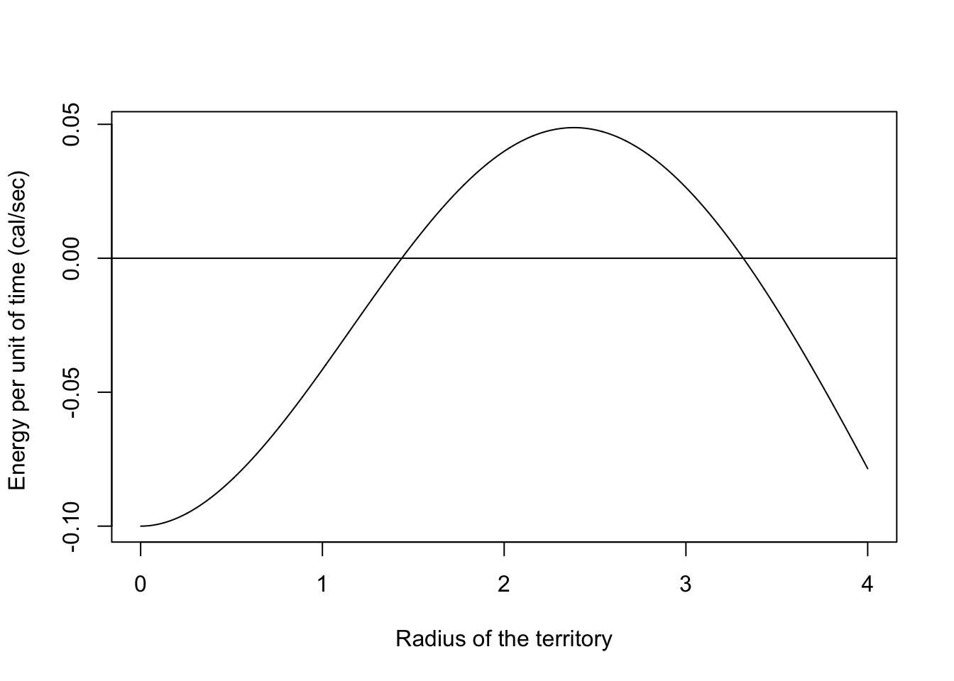
If you wanna read about an empirical test of this model, I suggest the paper by Shaffir and Rougharden [@-shafir1998].
2.3 Does natural selection maximizes fitness?
Simple models of population genetics for frequency independent selection.
Something on Tinberger, Konrad Lorenz on the genetic basis of behavior
2.4 Statistical confrontation: finding the maximum
- Explain how to find the maximum of a function with R. Parallel between genetic algorithms and optimization.