install.packages("rdryad")Appendix C — Tutorials to support computational labs
C.1 Plotting real life ecophysiological from Anolis lizards
By Andres Marmol
Why anoles? Anoles are among the most studied reptile organisms. They are vastly diverse with more than 488 species described until today — circa 11% of all the squamates without considering snakes — due to their outstanding adaptive radiation, which has inspired many to dive-in-depth into understanding how evolution has operated within this group (Lizards in an Evolutionary Tree by J. B. Losos is a highly recommended instructive reading for more info). As a result, very detailed data sets on many species of anoles, including information on micro habitat, field body temperature, activity patterns and morphological traits, performance, etc., can be found online in relatively few time.
In the following steps we will be downloading from Dryad and using a data set created by Winchell et al. (2016) (https://doi.org/10.5061/dryad.h234n) on Anolis cristatellus making a pair-comparison of several morphological and thermal traits of individuals living in urban and forested areas at Puerto Rico. A. cristatellus is widely distributed across Puerto Rico and can be found in natural and human-intervened spaces easily. It can be seen over ground and laying on the trunks of trees in natural settings, and on walls and metal fences in more urban areas.
C.1.1 Calling the dataset from Dryad
To download the dataset, it is necessary to install the R package rdryad.
Then we open the newly installed package and download the dataset by specifying the DOI associated to this dataset.
#calling rdryad
library(rdryad)

# Specify the DOI
doi <- "10.5061/dryad.h234n"

# Download the dataset using the dryad_download function
downloaded_file <- dryad_download(dois = doi)
The data sets are now downloaded on the paths indicated in the box below, although for this exercise only table [2] winchell_evol_phenshifts.csv” is needed.
# The downloaded_file will contain the file path where the dataset is saved
print(downloaded_file)
$`10.5061/dryad.h234n`
[1] "/Users/henrique/Library/Caches/R/rdryad/10_5061_dryad_h234n/winchell_evol_CG.csv"
[2] "/Users/henrique/Library/Caches/R/rdryad/10_5061_dryad_h234n/winchell_evol_phenshifts.csv"Once this is done, it is always good practice to check if the recently open data frame works by checking the columns within the data frame.
#calling the dataset of interest as df
df <- read.csv(downloaded_file[[1]][2])

# checking the columns (variables) available in the data frame df using the str function
names(df)
[1] "ID" "date" "Site"
[4] "context" "perch" "bodytemp.C"
[7] "perch.temp.C" "ambient.temp.C" "humidity.percent"
[10] "perch.height.cm" "perch.diam.cm" "weight.g"
[13] "head.height.mm" "svl.mm" "local.time.decimal"
[16] "flags" "JL" "JW"
[19] "METC" "RAD" "ULN"
[22] "HUM" "FEM" "TIB"
[25] "FIB" "METT1" "METT2"
[28] "FL" "HL" There are 29 different variables within df, but this exercise will focus only in a few of them including context, perch, bodytemp.C, perch.temp.C, ambient.temp.C, and local.time.decimal where context indicates if the lizard was captured in natural or urban spaces; perch refers to the microhabitat where the lizard was found; bodytemp.C is body temperature \(b\); perch.temp.C is substrate temperature \(T_s\); ambient.temp.C is air temperature \(a\); and local.time.decimal is the time of the day in hours when the lizards was captured and measured.
C.1.2 Exploring the thermophysiological data of A. cristatellus.
As covered in the first chapter, \(b\) increases proportionally to \(a\) as indicated in equation (1.2). Let’s check if the data confirms this equation.
# to call a variable directly from a data frame one must use $, indicating the name of the dataframe at the left and the name of the variable (columnt on the right).

plot(df$ambient.temp.C, df$bodytemp.C,
     xlab="air temperature (°C)",
     ylab="body temperature (°C)")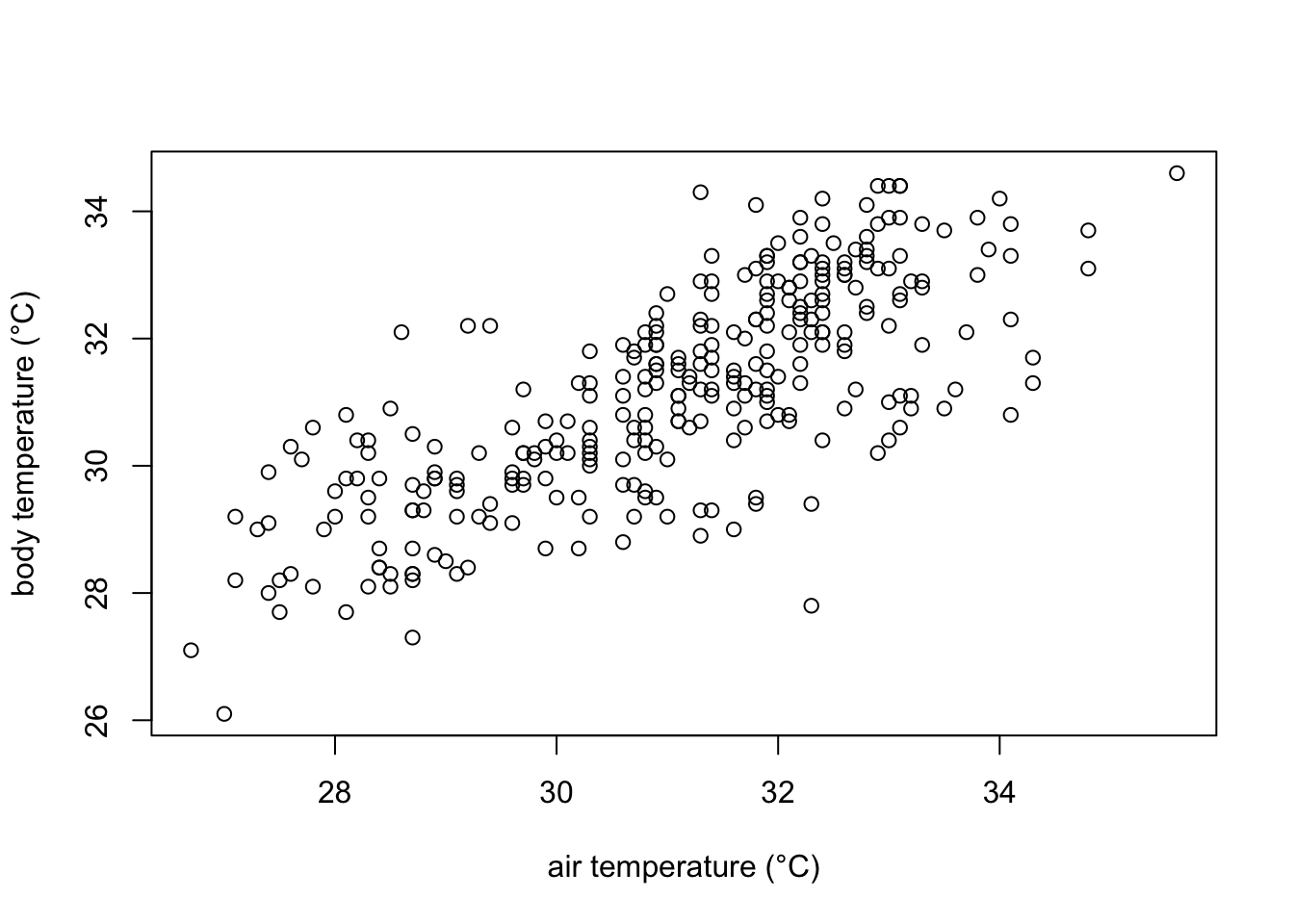
In the plot we can observe that indeed body temperature increases with increasing temperature. However, we cannot quantitatively know how much is this increase. For that, we can model how air temperature affects body temperature modelling them a a line with the equation:
\[ \hat{y} = α + β*x + e \tag{C.1}\] where \(\hat{y}\) is the predicted value of \(y\) for any given \(x\); \(α\) is point of intersection of the line when \(x=0\), \(β\) is the slope of the regression line (i.e. how much increases \(\hat{y}\) with a unit increase in \(x\)) and \(e\) is the random error.
Placing our variables in formula, it would look like this:
\[ b = b_{0} + β*a + e \tag{C.2}\]
where \(b\) is body temperature, \(a\) is ambient temperature, and \(b_0\) is the body temperature when \(a\) is zero.
Now lets model it using a least-squares linear regression using the lm function in R.
#define the linear model
#the variable at the left of the tilde (~) is the dependent variable
#data calls the specific dataframe to be used.

model1 <- lm(bodytemp.C ~ ambient.temp.C, data=df)

# print model outputs
print(model1)
Call:
lm(formula = bodytemp.C ~ ambient.temp.C, data = df)

Coefficients:
   (Intercept)  ambient.temp.C
        8.7004          0.7237
C.1.3 Interpreting the results of our model.
The results of our model indicates that if the air temperature (\(a\)) is zero, A. cristatellus would show a body temperature (\(b\)) of 8.7 °C, which increases in approximately 0.7 °C for each 1 °C increase in air temperature.
Now it is also possible to draw a few predictions
# a number of possible ambient temperatures that can be found in Puerto Rico during the day

amb_temps = data.frame(ambient.temp.C = seq(27,38, 1))# defines a vector with values from 27 to 38, with one unit increase

predict(model1, newdata=amb_temps)
1 2 3 4 5 6 7 8
28.23967 28.96335 29.68702 30.41070 31.13437 31.85805 32.58172 33.30540
9 10 11 12
34.02907 34.75275 35.47642 36.20010 C.2 How good our model is performing?
Graphically the linear model fits the data as follows:
# Create the scatter plot
plot(df$ambient.temp.C, df$bodytemp.C,
     xlab="air temperature (°C)",
     ylab="body temperature (°C)")

# add the line of fit from our recently created linear model "model1"
abline(model1, col = "red", lwd= 2)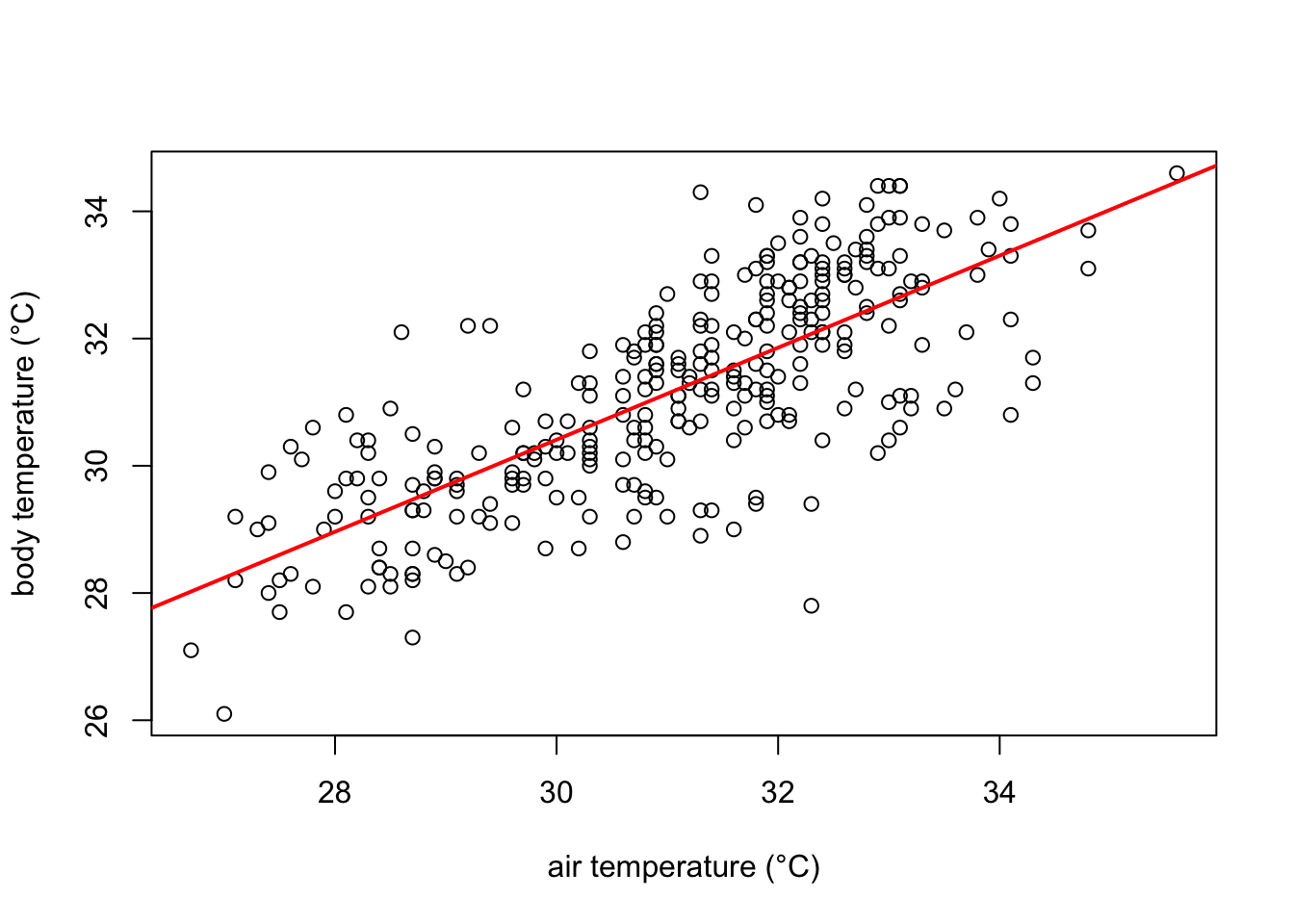
The red line in the plot follows very well the pattern of increase shown by our data. It is noticeable, however, that some points fall farther from the line of best fit than others. In other words, many \(\hat{y}\) values (body temperature) are predicted with larger errors than others, for a given \(x\) value (ambient temperature). These errors are also known as residuals, and are the vertical distance between the observed values and the line of best fit. They are graphically represented in green in our plot:
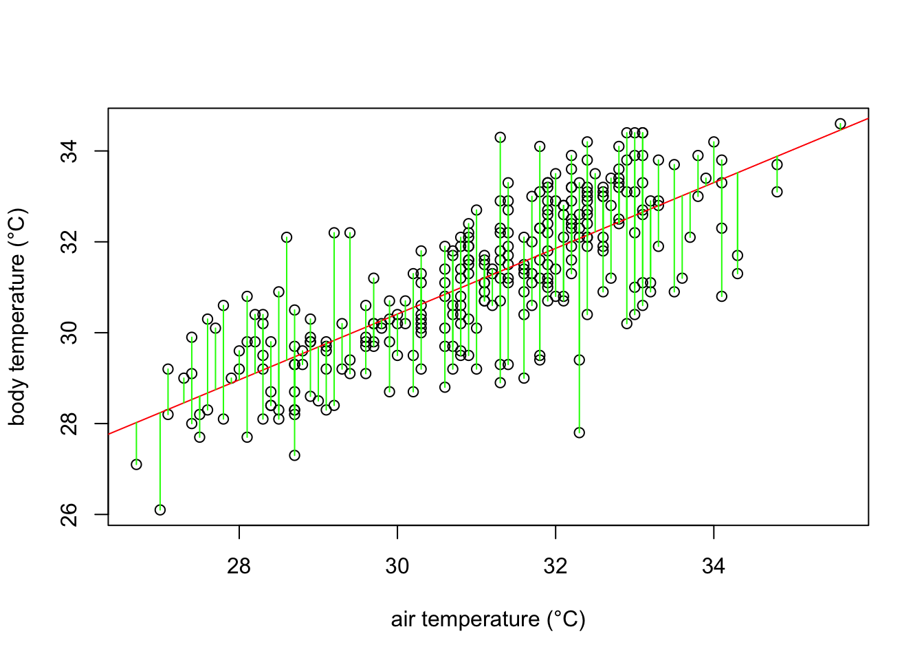
What a least square linear regression does is to find the lowest sum of squares of the residuals (every green line in the plot) so that the least amount of error is kept in the linear model.
Finally, how well the model fits the data? In our example, the body temperatures do not perfectly fall on the line of best fit, and many of them are scattered around it. A common metric assess this question in a simple regression model is the \(r^2\). \(r^2\) values indicates how much of the variance of body temperature (our dependent variable) is explained by ambient temperature (our independent variable). A perfect fit is indicated by an \(r^2\) of 1, while no fit would be zero. To check the \(r^2\) in our model we can simply use the summary function in R.
# obtaining the r-squared of our model

summary(model1)$r.squared
[1] 0.5736088\(r^2\) equals 0.574 indicating that almost 60% of the variance in body temperature is explained by ambient temperature.
In summary, our expectation that lizards body temperature increases depending on how the temperature in their environment changes has been confirmed. Specifically for A. cristatellus in this study, body temperature increases ~ 0.7 °C every 1 degree increase in air temperature. A few questions remain. For example, does habitat has an effect in the body temperature in A. cristatellus, and if it does, how different could the body temperatures of the lizards in habitat A are from those in habitat B?