Appendix A — A brief R tutorial

🚧 This chapter is under construction. Content may change.

If you are new to R you can have a short dive into its main features by working through this tutorial. If you had learnt programming in another computer language, you will be able to skim over this tutorial to find the main differences from what you have learnt to how things are done in R.

A.1 Basic data structures

A.1.1 Variables

Variables can be any sequence of letter and numbers, but # it cannot start with a number

x = 2
x <- 4
2+2

[1] 4

y <- x^5
y

[1] 1024

Please note that you can comment code by using the # character.

A.1.2 Vectors

Let’s create vectors.

# Introduction to vectors
v1 <- c(2,3,6,12)
v2 <- 1:100
length(v2)

[1] 100

v2

  [1]   1   2   3   4   5   6   7   8   9  10  11  12  13  14  15  16  17  18
 [19]  19  20  21  22  23  24  25  26  27  28  29  30  31  32  33  34  35  36
 [37]  37  38  39  40  41  42  43  44  45  46  47  48  49  50  51  52  53  54
 [55]  55  56  57  58  59  60  61  62  63  64  65  66  67  68  69  70  71  72
 [73]  73  74  75  76  77  78  79  80  81  82  83  84  85  86  87  88  89  90
 [91]  91  92  93  94  95  96  97  98  99 100

v3 <- seq(1,100,5)  # call without naming arguments
v3

 [1]  1  6 11 16 21 26 31 36 41 46 51 56 61 66 71 76 81 86 91 96

v3 <- seq(from=1,to=100,by=5) # call with names of arguments
v3

 [1]  1  6 11 16 21 26 31 36 41 46 51 56 61 66 71 76 81 86 91 96

v3 <- seq(to=100,by=5) # call skipping the first argument
#and using the default value 1 - see help(seq)
v3

 [1]  1  6 11 16 21 26 31 36 41 46 51 56 61 66 71 76 81 86 91 96

v3 <- seq(by=5,to=100) # call by arguments and change order or arguments

How to index vectors?

# Indexing vectors
v3[3] #uses square brackets to obtain the third element of the vector

[1] 11

v3>20 # produce a vector of boolean values that are TRUE when

 [1] FALSE FALSE FALSE FALSE  TRUE  TRUE  TRUE  TRUE  TRUE  TRUE  TRUE  TRUE
[13]  TRUE  TRUE  TRUE  TRUE  TRUE  TRUE  TRUE  TRUE

      #v3 is greater than 20
v3[v3>20] # select from v3 all the values that are greater than 20

 [1] 21 26 31 36 41 46 51 56 61 66 71 76 81 86 91 96

v4<-c(1,2,3,4,5)
v4[c(FALSE,TRUE,FALSE,TRUE,FALSE)] #select from v4 the second and fourth element

[1] 2 4

v3[1:10] # first ten elements

 [1]  1  6 11 16 21 26 31 36 41 46

v3[-1] # dropping first element

 [1]  6 11 16 21 26 31 36 41 46 51 56 61 66 71 76 81 86 91 96

head(v2) # prints the first few elements of v2

[1] 1 2 3 4 5 6

tail(v2) # prints the last few elements of v2

[1]  95  96  97  98  99 100

which(v3 == 26) # returns the position of v3 that equals 26

[1] 6

What kind of numerical operations are possible on vectors?

2^v2

  [1] 2.000000e+00 4.000000e+00 8.000000e+00 1.600000e+01 3.200000e+01
  [6] 6.400000e+01 1.280000e+02 2.560000e+02 5.120000e+02 1.024000e+03
 [11] 2.048000e+03 4.096000e+03 8.192000e+03 1.638400e+04 3.276800e+04
 [16] 6.553600e+04 1.310720e+05 2.621440e+05 5.242880e+05 1.048576e+06
 [21] 2.097152e+06 4.194304e+06 8.388608e+06 1.677722e+07 3.355443e+07
 [26] 6.710886e+07 1.342177e+08 2.684355e+08 5.368709e+08 1.073742e+09
 [31] 2.147484e+09 4.294967e+09 8.589935e+09 1.717987e+10 3.435974e+10
 [36] 6.871948e+10 1.374390e+11 2.748779e+11 5.497558e+11 1.099512e+12
 [41] 2.199023e+12 4.398047e+12 8.796093e+12 1.759219e+13 3.518437e+13
 [46] 7.036874e+13 1.407375e+14 2.814750e+14 5.629500e+14 1.125900e+15
 [51] 2.251800e+15 4.503600e+15 9.007199e+15 1.801440e+16 3.602880e+16
 [56] 7.205759e+16 1.441152e+17 2.882304e+17 5.764608e+17 1.152922e+18
 [61] 2.305843e+18 4.611686e+18 9.223372e+18 1.844674e+19 3.689349e+19
 [66] 7.378698e+19 1.475740e+20 2.951479e+20 5.902958e+20 1.180592e+21
 [71] 2.361183e+21 4.722366e+21 9.444733e+21 1.888947e+22 3.777893e+22
 [76] 7.555786e+22 1.511157e+23 3.022315e+23 6.044629e+23 1.208926e+24
 [81] 2.417852e+24 4.835703e+24 9.671407e+24 1.934281e+25 3.868563e+25
 [86] 7.737125e+25 1.547425e+26 3.094850e+26 6.189700e+26 1.237940e+27
 [91] 2.475880e+27 4.951760e+27 9.903520e+27 1.980704e+28 3.961408e+28
 [96] 7.922816e+28 1.584563e+29 3.169127e+29 6.338253e+29 1.267651e+30

log(v2)

  [1] 0.0000000 0.6931472 1.0986123 1.3862944 1.6094379 1.7917595 1.9459101
  [8] 2.0794415 2.1972246 2.3025851 2.3978953 2.4849066 2.5649494 2.6390573
 [15] 2.7080502 2.7725887 2.8332133 2.8903718 2.9444390 2.9957323 3.0445224
 [22] 3.0910425 3.1354942 3.1780538 3.2188758 3.2580965 3.2958369 3.3322045
 [29] 3.3672958 3.4011974 3.4339872 3.4657359 3.4965076 3.5263605 3.5553481
 [36] 3.5835189 3.6109179 3.6375862 3.6635616 3.6888795 3.7135721 3.7376696
 [43] 3.7612001 3.7841896 3.8066625 3.8286414 3.8501476 3.8712010 3.8918203
 [50] 3.9120230 3.9318256 3.9512437 3.9702919 3.9889840 4.0073332 4.0253517
 [57] 4.0430513 4.0604430 4.0775374 4.0943446 4.1108739 4.1271344 4.1431347
 [64] 4.1588831 4.1743873 4.1896547 4.2046926 4.2195077 4.2341065 4.2484952
 [71] 4.2626799 4.2766661 4.2904594 4.3040651 4.3174881 4.3307333 4.3438054
 [78] 4.3567088 4.3694479 4.3820266 4.3944492 4.4067192 4.4188406 4.4308168
 [85] 4.4426513 4.4543473 4.4659081 4.4773368 4.4886364 4.4998097 4.5108595
 [92] 4.5217886 4.5325995 4.5432948 4.5538769 4.5643482 4.5747110 4.5849675
 [99] 4.5951199 4.6051702

v5 <- 101:200
v5/v2

  [1] 101.000000  51.000000  34.333333  26.000000  21.000000  17.666667
  [7]  15.285714  13.500000  12.111111  11.000000  10.090909   9.333333
 [13]   8.692308   8.142857   7.666667   7.250000   6.882353   6.555556
 [19]   6.263158   6.000000   5.761905   5.545455   5.347826   5.166667
 [25]   5.000000   4.846154   4.703704   4.571429   4.448276   4.333333
 [31]   4.225806   4.125000   4.030303   3.941176   3.857143   3.777778
 [37]   3.702703   3.631579   3.564103   3.500000   3.439024   3.380952
 [43]   3.325581   3.272727   3.222222   3.173913   3.127660   3.083333
 [49]   3.040816   3.000000   2.960784   2.923077   2.886792   2.851852
 [55]   2.818182   2.785714   2.754386   2.724138   2.694915   2.666667
 [61]   2.639344   2.612903   2.587302   2.562500   2.538462   2.515152
 [67]   2.492537   2.470588   2.449275   2.428571   2.408451   2.388889
 [73]   2.369863   2.351351   2.333333   2.315789   2.298701   2.282051
 [79]   2.265823   2.250000   2.234568   2.219512   2.204819   2.190476
 [85]   2.176471   2.162791   2.149425   2.136364   2.123596   2.111111
 [91]   2.098901   2.086957   2.075269   2.063830   2.052632   2.041667
 [97]   2.030928   2.020408   2.010101   2.000000

A.1.3 Strings

#Using strings in R
mystring <- "Ecology"
vstrg <- c("Anna", "Peter", "Xavier")
vstrg[2]

[1] "Peter"

A.1.4 Matrices

m <- matrix(5,3,2)
m

     [,1] [,2]
[1,]    5    5
[2,]    5    5
[3,]    5    5

m2 <- matrix(1:6,3,2)
m2

     [,1] [,2]
[1,]    1    4
[2,]    2    5
[3,]    3    6

t(m2) # transposes matrix

     [,1] [,2] [,3]
[1,]    1    2    3
[2,]    4    5    6

x <- 1:4
y <- 5:8

m3<-cbind(x,y)
m3

     x y
[1,] 1 5
[2,] 2 6
[3,] 3 7
[4,] 4 8

m4<-rbind(x,y)
m4

  [,1] [,2] [,3] [,4]
x    1    2    3    4
y    5    6    7    8

# Indexing matrices
m3[3,2] #element in row 3 and column 2

y 
7

m3[1,] #entire first row

x y 
1 5

m3[,1] #entire first column

[1] 1 2 3 4

colnames(m3)<-c("col1","col2")
m3

     col1 col2
[1,]    1    5
[2,]    2    6
[3,]    3    7
[4,]    4    8

m3[,"col2"]

[1] 5 6 7 8

A.1.5 Lists

# Lists in R
mylist <- list(elem1=m,elem2=v2,elem3="my list")
mylist$elem2

  [1]   1   2   3   4   5   6   7   8   9  10  11  12  13  14  15  16  17  18
 [19]  19  20  21  22  23  24  25  26  27  28  29  30  31  32  33  34  35  36
 [37]  37  38  39  40  41  42  43  44  45  46  47  48  49  50  51  52  53  54
 [55]  55  56  57  58  59  60  61  62  63  64  65  66  67  68  69  70  71  72
 [73]  73  74  75  76  77  78  79  80  81  82  83  84  85  86  87  88  89  90
 [91]  91  92  93  94  95  96  97  98  99 100

A.1.6 Dataframes

# Dataframes
df <- as.data.frame(m3)
df$col1

[1] 1 2 3 4

A.2 Basic plots in R

#making plots in R
plot(v2,v2)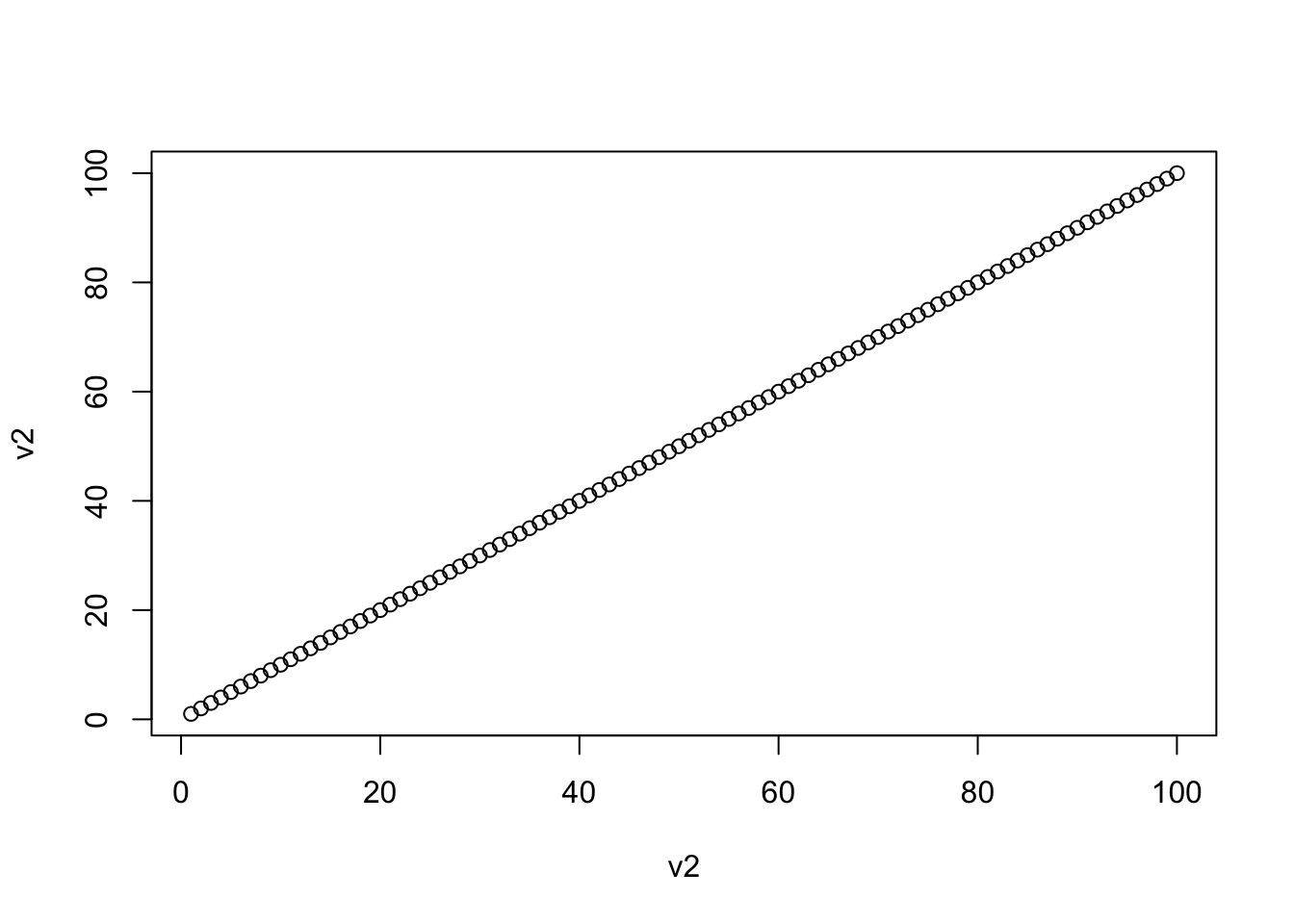

plot(v2,v2^2)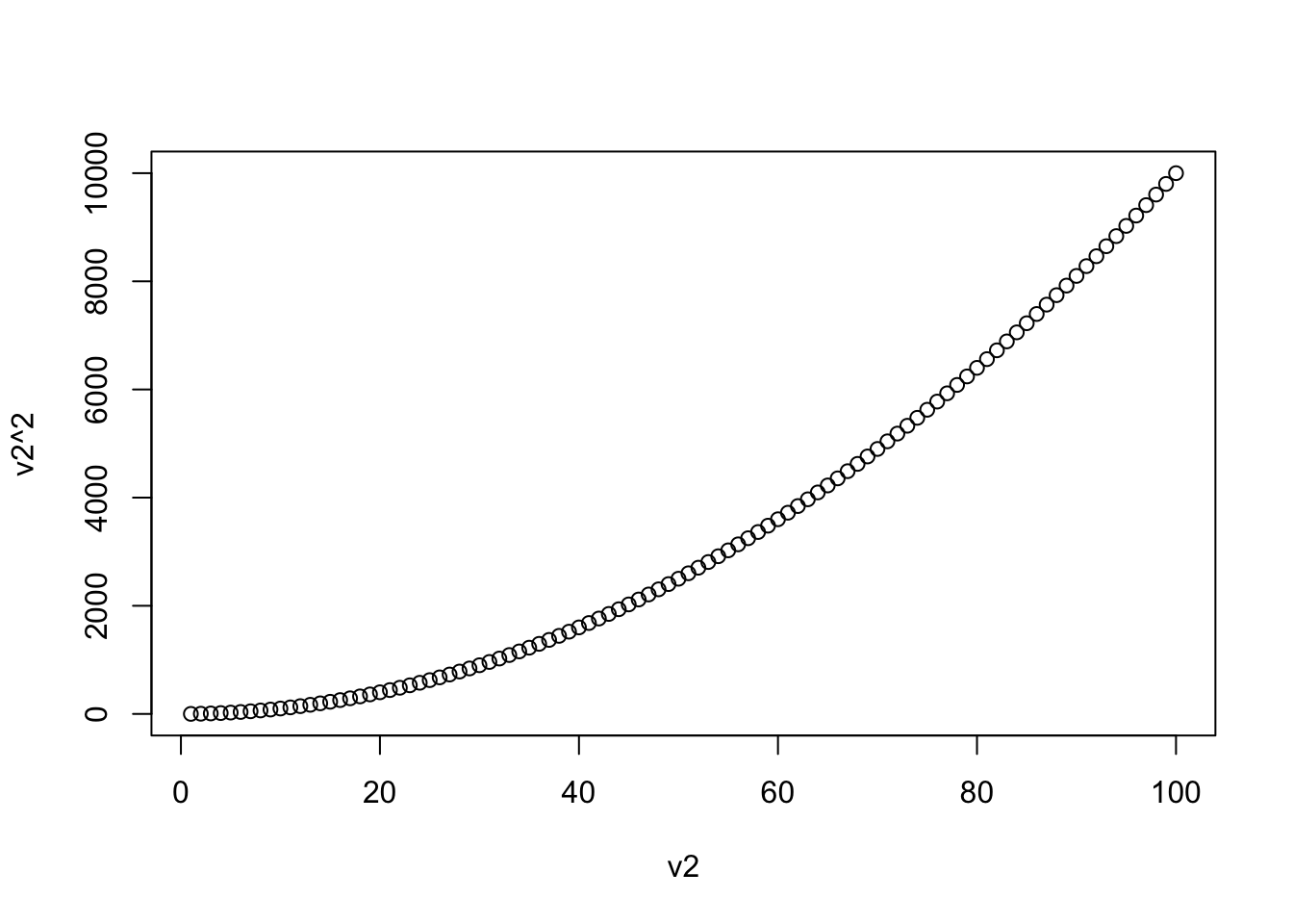

plot(v2,v2^2,type="l")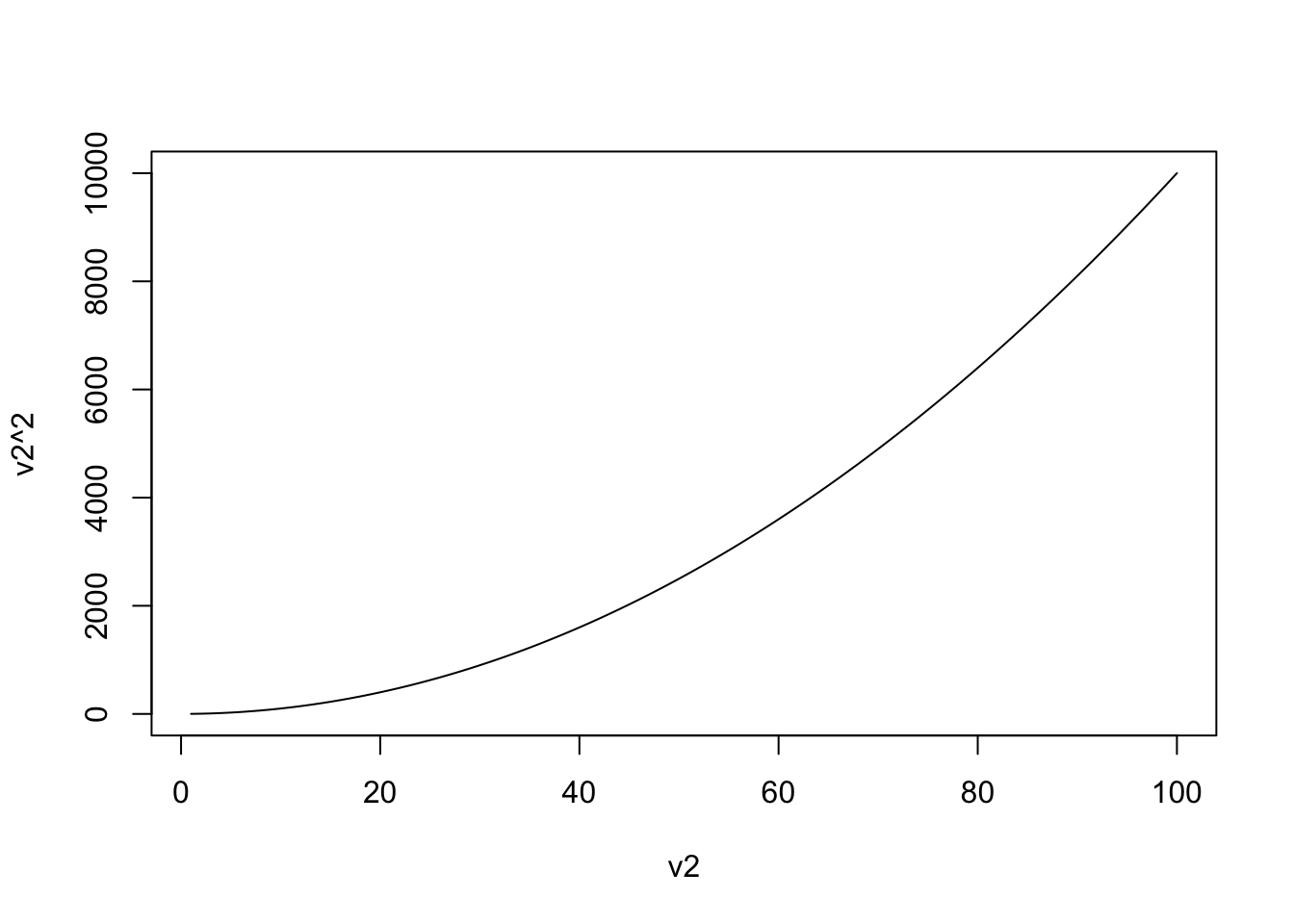

plot(v2,v2^2,type="l",col="red")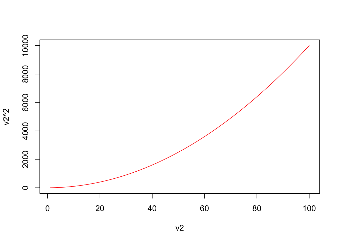

plot(v2,v2^2,type="l",col="red",main="My beautiful plot")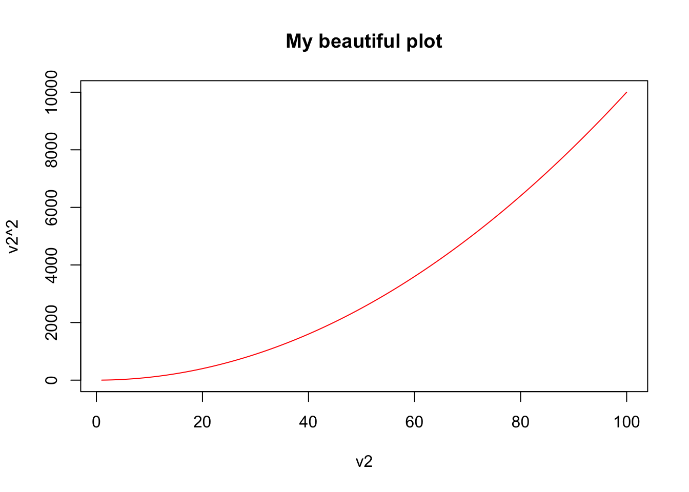

plot(v2,v2^2,type="l",col="red",main="My beautiful plot",xlab="x",
     ylab="x^2")
lines(v2,v2^3,col="blue")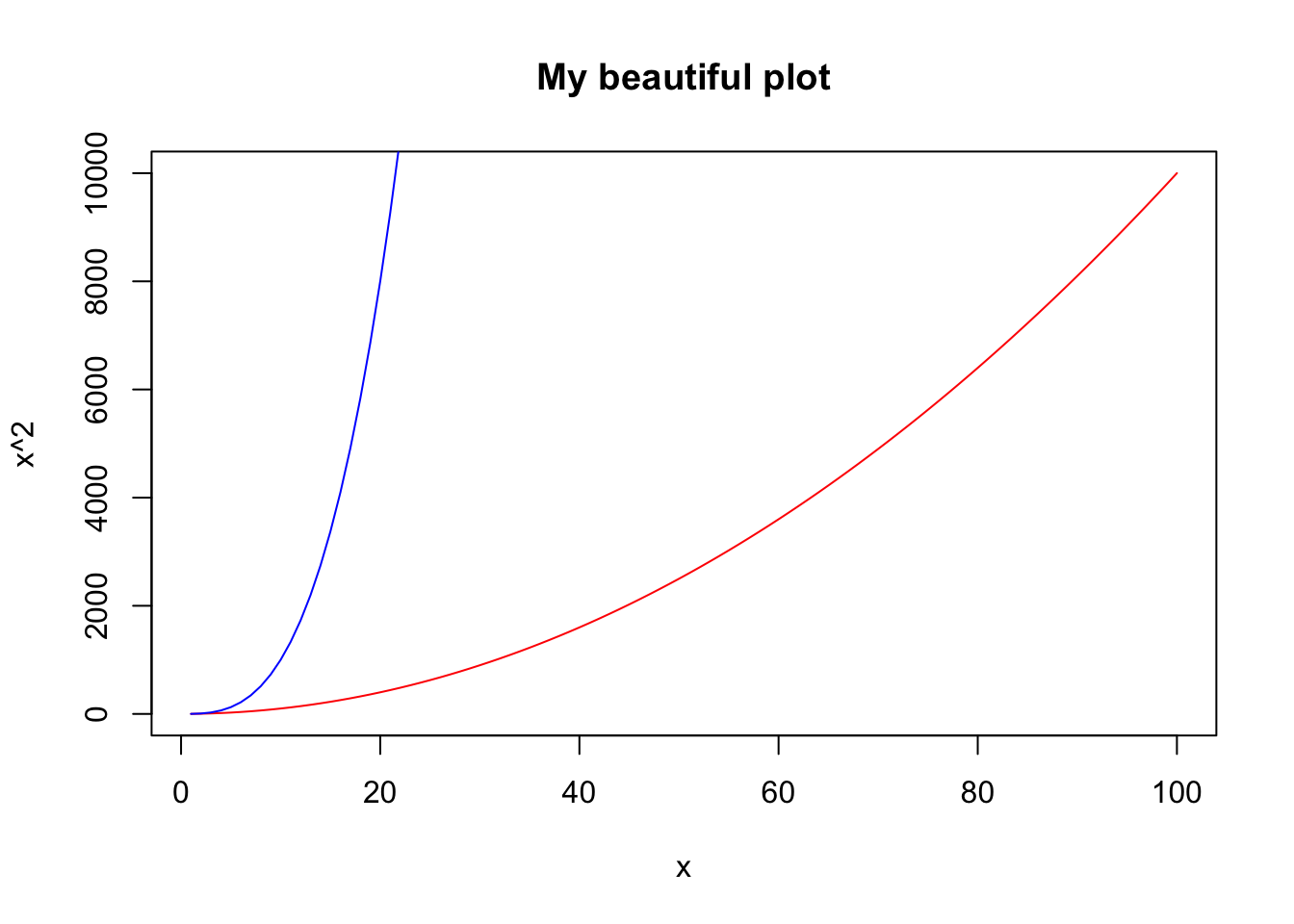

A.3 Iterations and conditional expressions

# FOR loops

for (k in 1:10)  # for k =1, 2, 3, 4, 5,...10
  print (k^2)   #do this

[1] 1
[1] 4
[1] 9
[1] 16
[1] 25
[1] 36
[1] 49
[1] 64
[1] 81
[1] 100

R <- 1.2
n <- 1
print(n[1])

[1] 1

for (t in 1:100)
{
  n[t+1] <- R*n[t]
  print(n[t+1])
}

[1] 1.2
[1] 1.44
[1] 1.728
[1] 2.0736
[1] 2.48832
[1] 2.985984
[1] 3.583181
[1] 4.299817
[1] 5.15978
[1] 6.191736
[1] 7.430084
[1] 8.9161
[1] 10.69932
[1] 12.83918
[1] 15.40702
[1] 18.48843
[1] 22.18611
[1] 26.62333
[1] 31.948
[1] 38.3376
[1] 46.00512
[1] 55.20614
[1] 66.24737
[1] 79.49685
[1] 95.39622
[1] 114.4755
[1] 137.3706
[1] 164.8447
[1] 197.8136
[1] 237.3763
[1] 284.8516
[1] 341.8219
[1] 410.1863
[1] 492.2235
[1] 590.6682
[1] 708.8019
[1] 850.5622
[1] 1020.675
[1] 1224.81
[1] 1469.772
[1] 1763.726
[1] 2116.471
[1] 2539.765
[1] 3047.718
[1] 3657.262
[1] 4388.714
[1] 5266.457
[1] 6319.749
[1] 7583.698
[1] 9100.438
[1] 10920.53
[1] 13104.63
[1] 15725.56
[1] 18870.67
[1] 22644.8
[1] 27173.76
[1] 32608.52
[1] 39130.22
[1] 46956.26
[1] 56347.51
[1] 67617.02
[1] 81140.42
[1] 97368.5
[1] 116842.2
[1] 140210.6
[1] 168252.8
[1] 201903.3
[1] 242284
[1] 290740.8
[1] 348889
[1] 418666.7
[1] 502400.1
[1] 602880.1
[1] 723456.1
[1] 868147.4
[1] 1041777
[1] 1250132
[1] 1500159
[1] 1800190
[1] 2160228
[1] 2592274
[1] 3110729
[1] 3732875
[1] 4479450
[1] 5375340
[1] 6450408
[1] 7740489
[1] 9288587
[1] 11146304
[1] 13375565
[1] 16050678
[1] 19260814
[1] 23112977
[1] 27735572
[1] 33282687
[1] 39939224
[1] 47927069
[1] 57512482
[1] 69014979
[1] 82817975

R <- 1.2
n <- 1
for (t in 1:100)
  n[t+1] <- R*n[t]

# IF conditional statement

# logical operators
# == equal to
# > greater than
# < smaller than
# >= greater or equal
# <= smaller or equal
# != different from
# && and
# || or

if (3>2) print ("yes")

[1] "yes"

if (3==2) print ("yes") else print("no")

[1] "no"

if ((3>2)&&(4>5)) print ("yes")

for (k in 1:10)  # for k =1, 2, 3, 4, 5,...10
  if (k^2>20) print (k^2)

[1] 25
[1] 36
[1] 49
[1] 64
[1] 81
[1] 100

A.4 Writing functions

# creating FUNCTIONS in r

pythagoras <- function (c1,c2)
{
  h <- sqrt (c1^2 + c2^2)
  return (h)
}

pythagoras(1,1)

[1] 1.414214

pythagoras(5,5)

[1] 7.071068

pythagoras(10,1)

[1] 10.04988

# regression in R

help(lm)
x <- c(1,2,3,4)
y <- c(1.1,2.3,2.9,4.1)
plot(x,y)
myreg<-lm(y ~ x)
summary(myreg)


Call:
lm(formula = y ~ x)

Residuals:
    1     2     3     4 
-0.06  0.18 -0.18  0.06 

Coefficients:
            Estimate Std. Error t value Pr(>|t|)   
(Intercept)  0.20000    0.23238   0.861  0.48012   
x            0.96000    0.08485  11.314  0.00772 **
---
Signif. codes:  0 '***' 0.001 '**' 0.01 '*' 0.05 '.' 0.1 ' ' 1

Residual standard error: 0.1897 on 2 degrees of freedom
Multiple R-squared:  0.9846,    Adjusted R-squared:  0.9769 
F-statistic:   128 on 1 and 2 DF,  p-value: 0.007722

abline(myreg)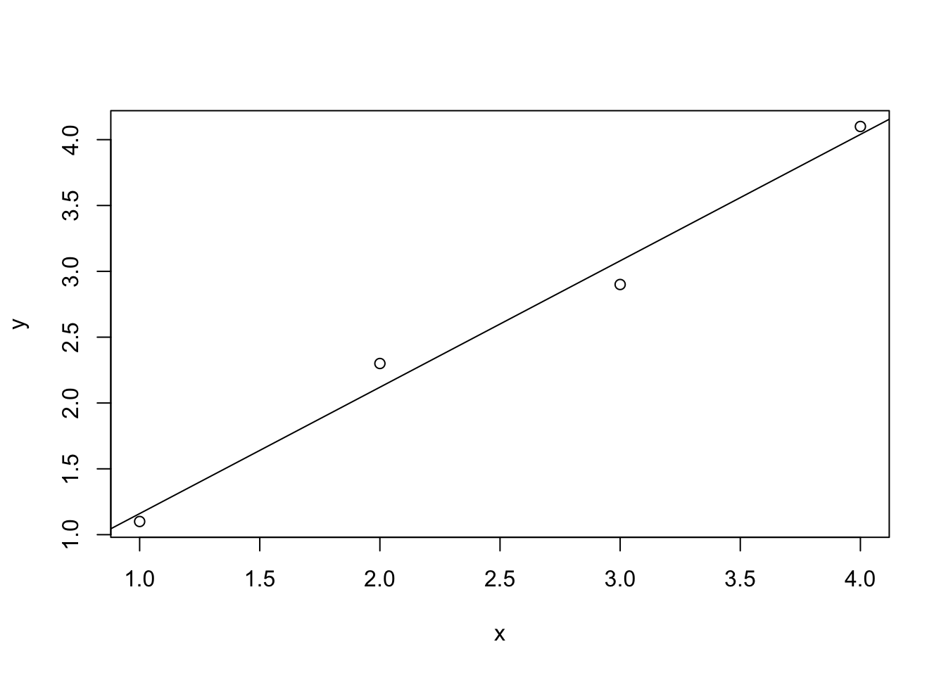

A.5 Random numbers and statistical distributions

random1d<-function(tmax)
{
x<-0
for (t in 1:tmax)
{
  r<-runif(1)
  if (r<1/2)
    x[t+1]<-x[t]+1 else
      x[t+1]<-x[t]-1
}
return(x)
}

plot(random1d(100))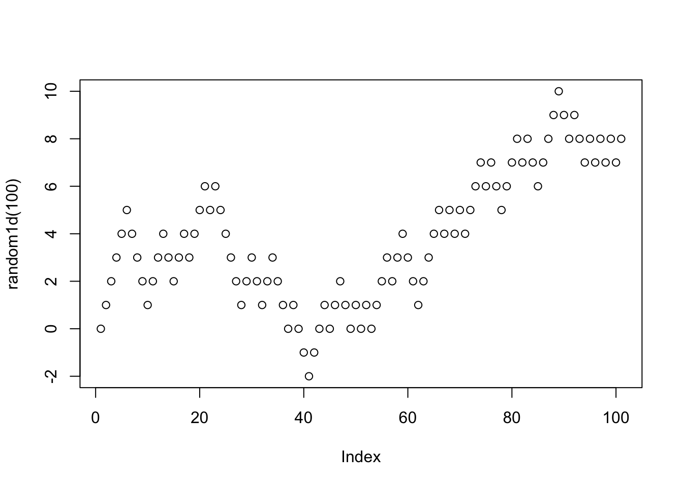

tmax<-10000
lastx<-0
for (i in 1:1000)
{
  x<-random1d(tmax)
  lastx[i]<-x[tmax]
}

hist(lastx)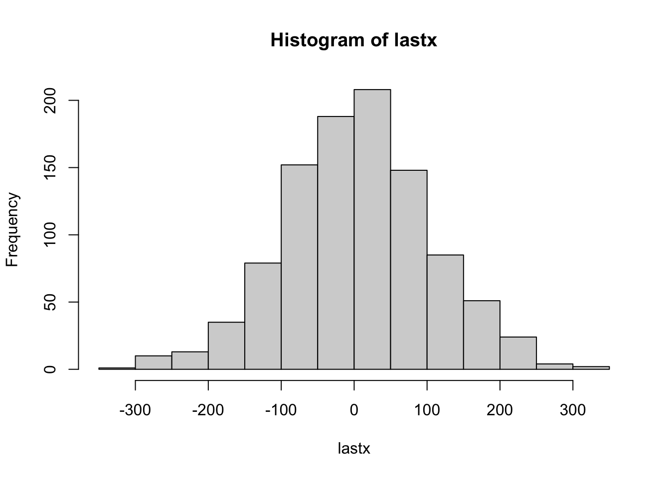

mean(lastx)

[1] 4.222

d<-sqrt(lastx^2)
hist(d)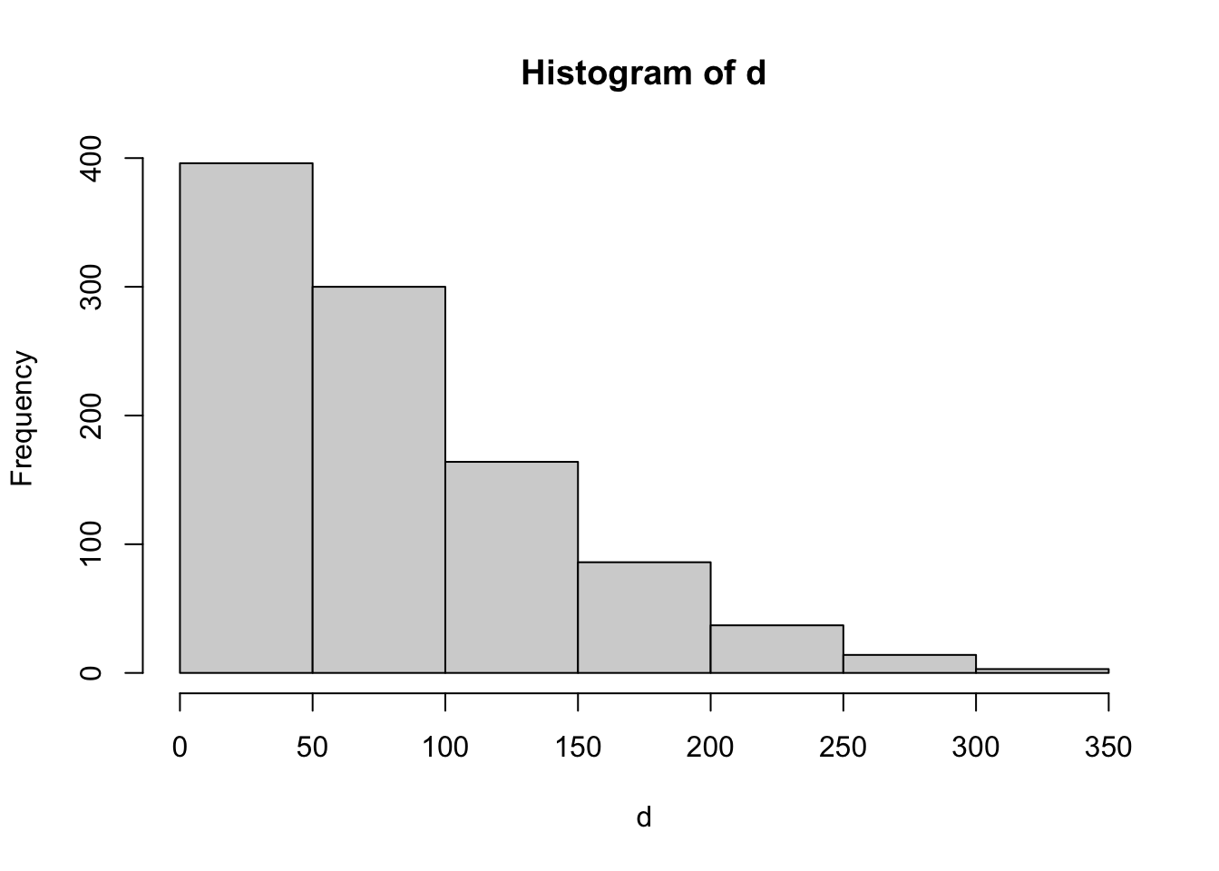

mean(d)

[1] 79.27

median(d)

[1] 65

max(d)

[1] 329

hist(d[d<20],breaks=c(1:20))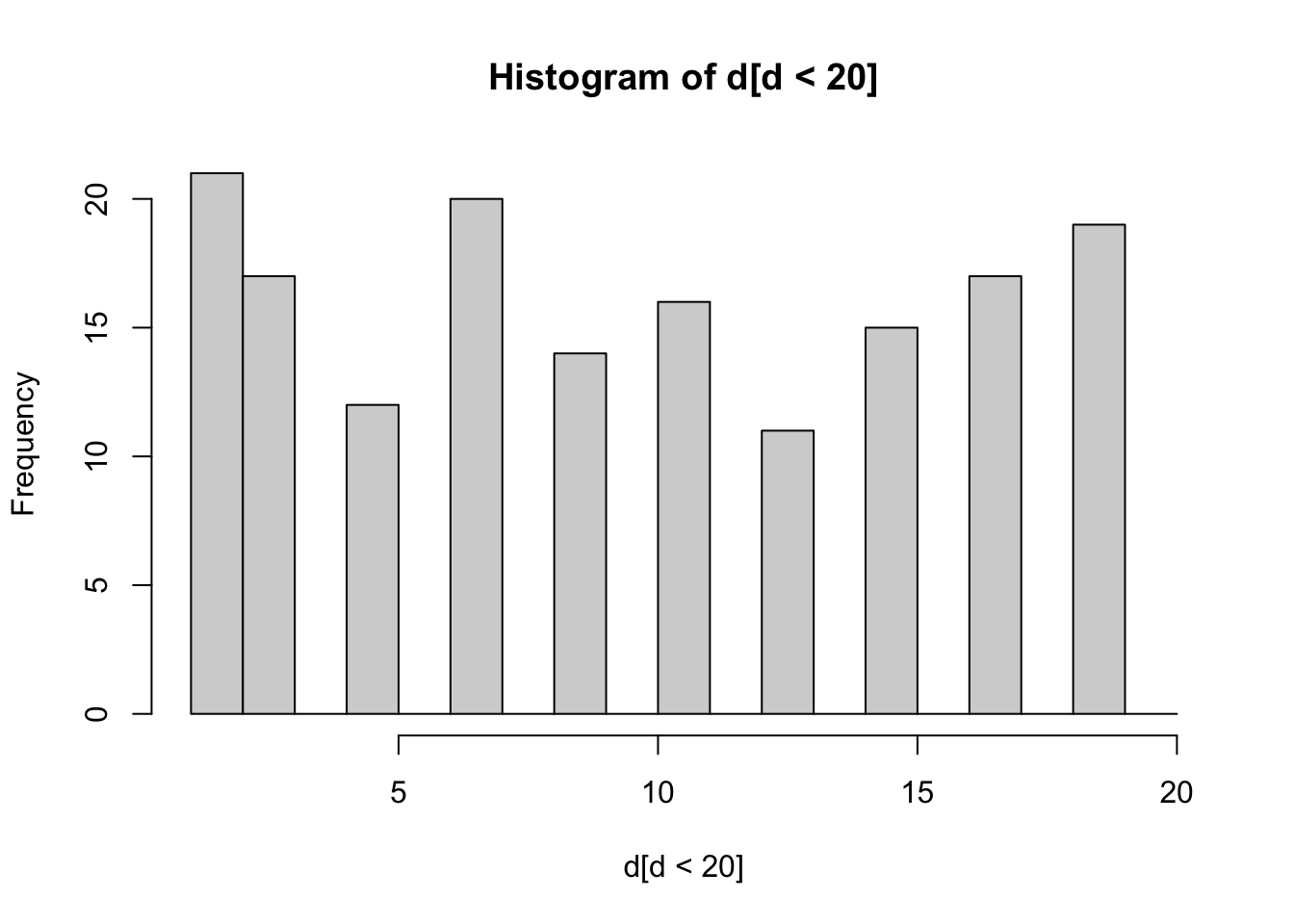

A.6 Intro to apply, pipes, ggplot2, tidyverse

Use of apply instead of for loops.

# a recursive function that calculates a factorial
myfun <- function(x)
{
  if (x==1)
    return (1)
  else return(x*myfun(x-1))
}

The following does not work

myfun(1:10) # does not work

One needs to do a for loop or use apply

#option1 - with a for loop
start_time <- Sys.time()
y<-0
for (i in 1:100)
  y[i]<-myfun(i)
end_time <- Sys.time()
end_time-start_time

Time difference of 0.009744167 secs

  [1]  1.000000e+00  2.000000e+00  6.000000e+00  2.400000e+01  1.200000e+02
  [6]  7.200000e+02  5.040000e+03  4.032000e+04  3.628800e+05  3.628800e+06
 [11]  3.991680e+07  4.790016e+08  6.227021e+09  8.717829e+10  1.307674e+12
 [16]  2.092279e+13  3.556874e+14  6.402374e+15  1.216451e+17  2.432902e+18
 [21]  5.109094e+19  1.124001e+21  2.585202e+22  6.204484e+23  1.551121e+25
 [26]  4.032915e+26  1.088887e+28  3.048883e+29  8.841762e+30  2.652529e+32
 [31]  8.222839e+33  2.631308e+35  8.683318e+36  2.952328e+38  1.033315e+40
 [36]  3.719933e+41  1.376375e+43  5.230226e+44  2.039788e+46  8.159153e+47
 [41]  3.345253e+49  1.405006e+51  6.041526e+52  2.658272e+54  1.196222e+56
 [46]  5.502622e+57  2.586232e+59  1.241392e+61  6.082819e+62  3.041409e+64
 [51]  1.551119e+66  8.065818e+67  4.274883e+69  2.308437e+71  1.269640e+73
 [56]  7.109986e+74  4.052692e+76  2.350561e+78  1.386831e+80  8.320987e+81
 [61]  5.075802e+83  3.146997e+85  1.982608e+87  1.268869e+89  8.247651e+90
 [66]  5.443449e+92  3.647111e+94  2.480036e+96  1.711225e+98 1.197857e+100
 [71] 8.504786e+101 6.123446e+103 4.470115e+105 3.307885e+107 2.480914e+109
 [76] 1.885495e+111 1.451831e+113 1.132428e+115 8.946182e+116 7.156946e+118
 [81] 5.797126e+120 4.753643e+122 3.945524e+124 3.314240e+126 2.817104e+128
 [86] 2.422710e+130 2.107757e+132 1.854826e+134 1.650796e+136 1.485716e+138
 [91] 1.352002e+140 1.243841e+142 1.156773e+144 1.087366e+146 1.032998e+148
 [96] 9.916779e+149 9.619276e+151 9.426890e+153 9.332622e+155 9.332622e+157

#option 2 - with apply
start_time <- Sys.time()
y<-sapply(1:100,myfun)
end_time <- Sys.time()
end_time-start_time

Time difference of 0.004185915 secs

  [1]  1.000000e+00  2.000000e+00  6.000000e+00  2.400000e+01  1.200000e+02
  [6]  7.200000e+02  5.040000e+03  4.032000e+04  3.628800e+05  3.628800e+06
 [11]  3.991680e+07  4.790016e+08  6.227021e+09  8.717829e+10  1.307674e+12
 [16]  2.092279e+13  3.556874e+14  6.402374e+15  1.216451e+17  2.432902e+18
 [21]  5.109094e+19  1.124001e+21  2.585202e+22  6.204484e+23  1.551121e+25
 [26]  4.032915e+26  1.088887e+28  3.048883e+29  8.841762e+30  2.652529e+32
 [31]  8.222839e+33  2.631308e+35  8.683318e+36  2.952328e+38  1.033315e+40
 [36]  3.719933e+41  1.376375e+43  5.230226e+44  2.039788e+46  8.159153e+47
 [41]  3.345253e+49  1.405006e+51  6.041526e+52  2.658272e+54  1.196222e+56
 [46]  5.502622e+57  2.586232e+59  1.241392e+61  6.082819e+62  3.041409e+64
 [51]  1.551119e+66  8.065818e+67  4.274883e+69  2.308437e+71  1.269640e+73
 [56]  7.109986e+74  4.052692e+76  2.350561e+78  1.386831e+80  8.320987e+81
 [61]  5.075802e+83  3.146997e+85  1.982608e+87  1.268869e+89  8.247651e+90
 [66]  5.443449e+92  3.647111e+94  2.480036e+96  1.711225e+98 1.197857e+100
 [71] 8.504786e+101 6.123446e+103 4.470115e+105 3.307885e+107 2.480914e+109
 [76] 1.885495e+111 1.451831e+113 1.132428e+115 8.946182e+116 7.156946e+118
 [81] 5.797126e+120 4.753643e+122 3.945524e+124 3.314240e+126 2.817104e+128
 [86] 2.422710e+130 2.107757e+132 1.854826e+134 1.650796e+136 1.485716e+138
 [91] 1.352002e+140 1.243841e+142 1.156773e+144 1.087366e+146 1.032998e+148
 [96] 9.916779e+149 9.619276e+151 9.426890e+153 9.332622e+155 9.332622e+157

Selecting a subset from a matrix and applying a function to a column of that subset

Florida <- read.csv("Labs/Florida.csv")

# number of species for year 1970 and route 20
x=tapply(Florida$Abundance,Florida$Route==20 & Florida$Year==1970, length)
#applies length() to Florida$Abundance but by two levels, when the formula is true
#and when the formula is false

# matrix with number of species per route and per year
out<-tapply(Florida$Abundance,list(Florida$Route,Florida$Year), length)

plot(out[10,])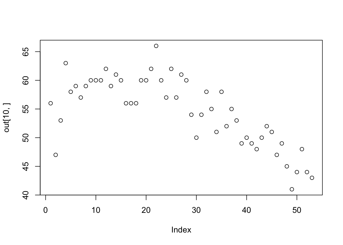

shannon<-function(x)
{
  p<-x/sum(x)
  - sum(p*log(p))
}

out<-tapply(Florida$Abundance,list(Florida$Route,Florida$Year), shannon)
plot(out[10,])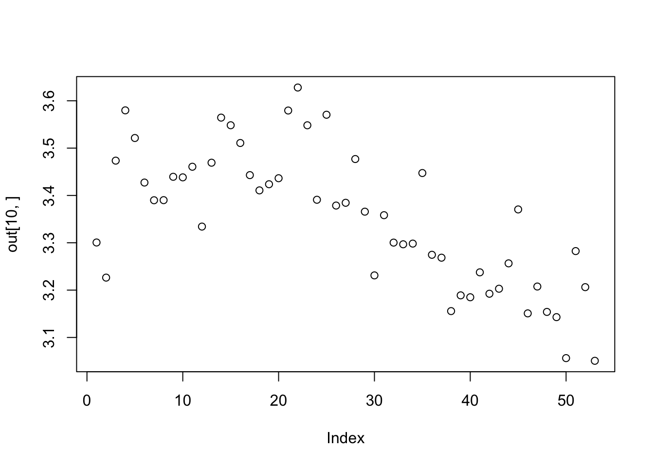

A.6.1 Working with pipes

library(tidyverse)

── Attaching core tidyverse packages ──────────────────────── tidyverse 2.0.0 ──
✔ dplyr     1.2.0     ✔ readr     2.1.5
✔ forcats   1.0.1     ✔ stringr   1.5.2
✔ ggplot2   4.0.0     ✔ tibble    3.3.0
✔ lubridate 1.9.4     ✔ tidyr     1.3.1
✔ purrr     1.2.1     
── Conflicts ────────────────────────────────────────── tidyverse_conflicts() ──
✖ dplyr::filter() masks stats::filter()
✖ dplyr::lag()    masks stats::lag()
ℹ Use the conflicted package (<http://conflicted.r-lib.org/>) to force all conflicts to become errors

#our first pipe
x<-rnorm(1000)
hist(x)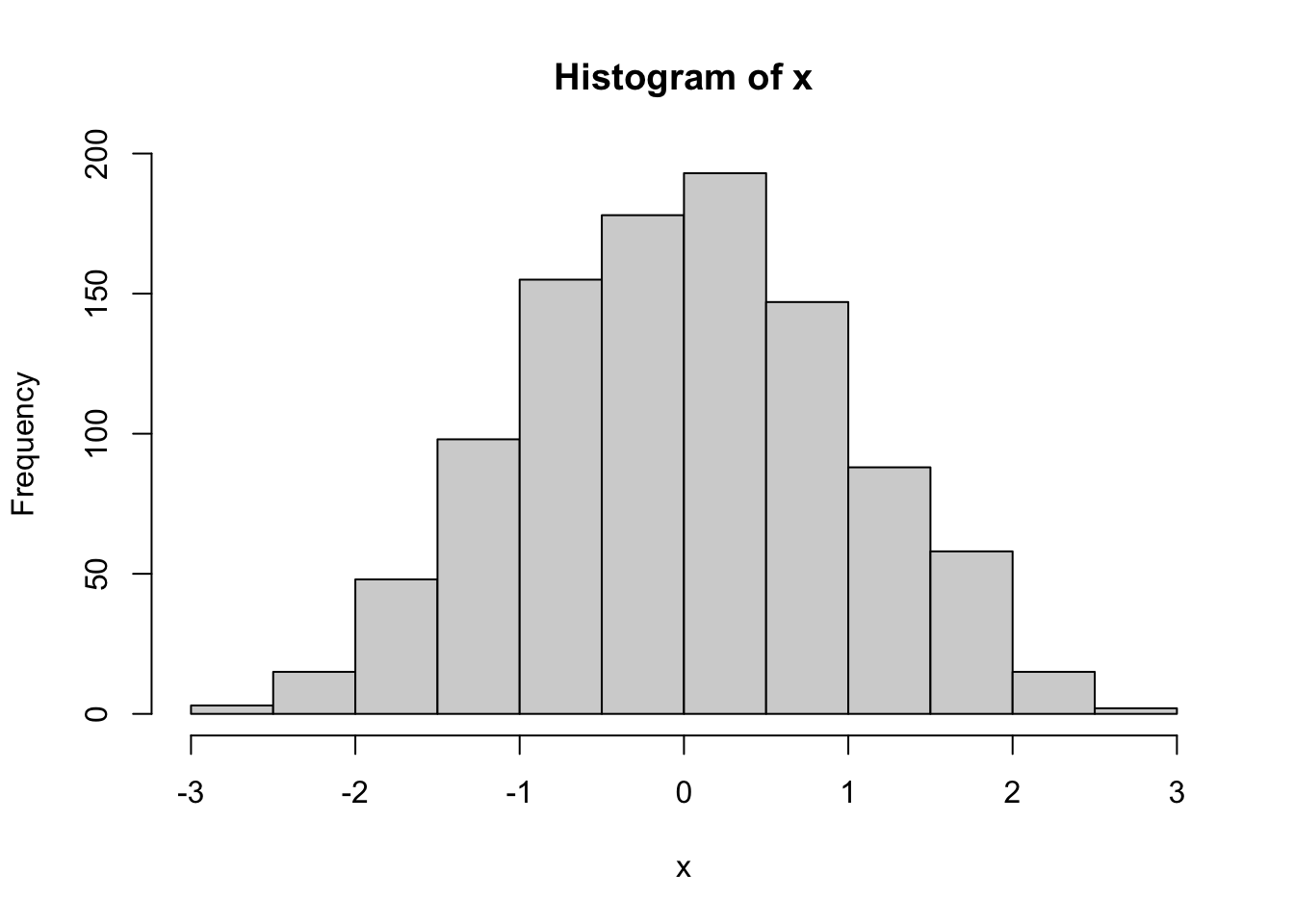

rnorm(1000) %>%  hist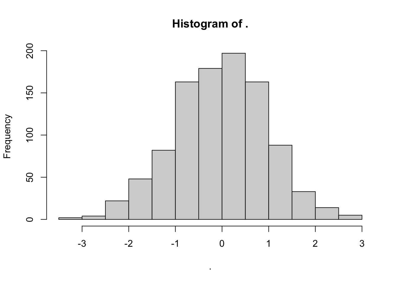

Now with the Florida data

t<-1:ncol(out)

plot(out[10,])
myreg<-lm(out[10,]~t)
summary(myreg)


Call:
lm(formula = out[10, ] ~ t)

Residuals:
      Min        1Q    Median        3Q       Max 
-0.289301 -0.062193 -0.007159  0.033154  0.243719 

Coefficients:
              Estimate Std. Error t value Pr(>|t|)    
(Intercept)  3.5288806  0.0289650  121.83  < 2e-16 ***
t           -0.0065709  0.0009334   -7.04 4.71e-09 ***
---
Signif. codes:  0 '***' 0.001 '**' 0.01 '*' 0.05 '.' 0.1 ' ' 1

Residual standard error: 0.1039 on 51 degrees of freedom
Multiple R-squared:  0.4928,    Adjusted R-squared:  0.4829 
F-statistic: 49.56 on 1 and 51 DF,  p-value: 4.708e-09

abline(myreg)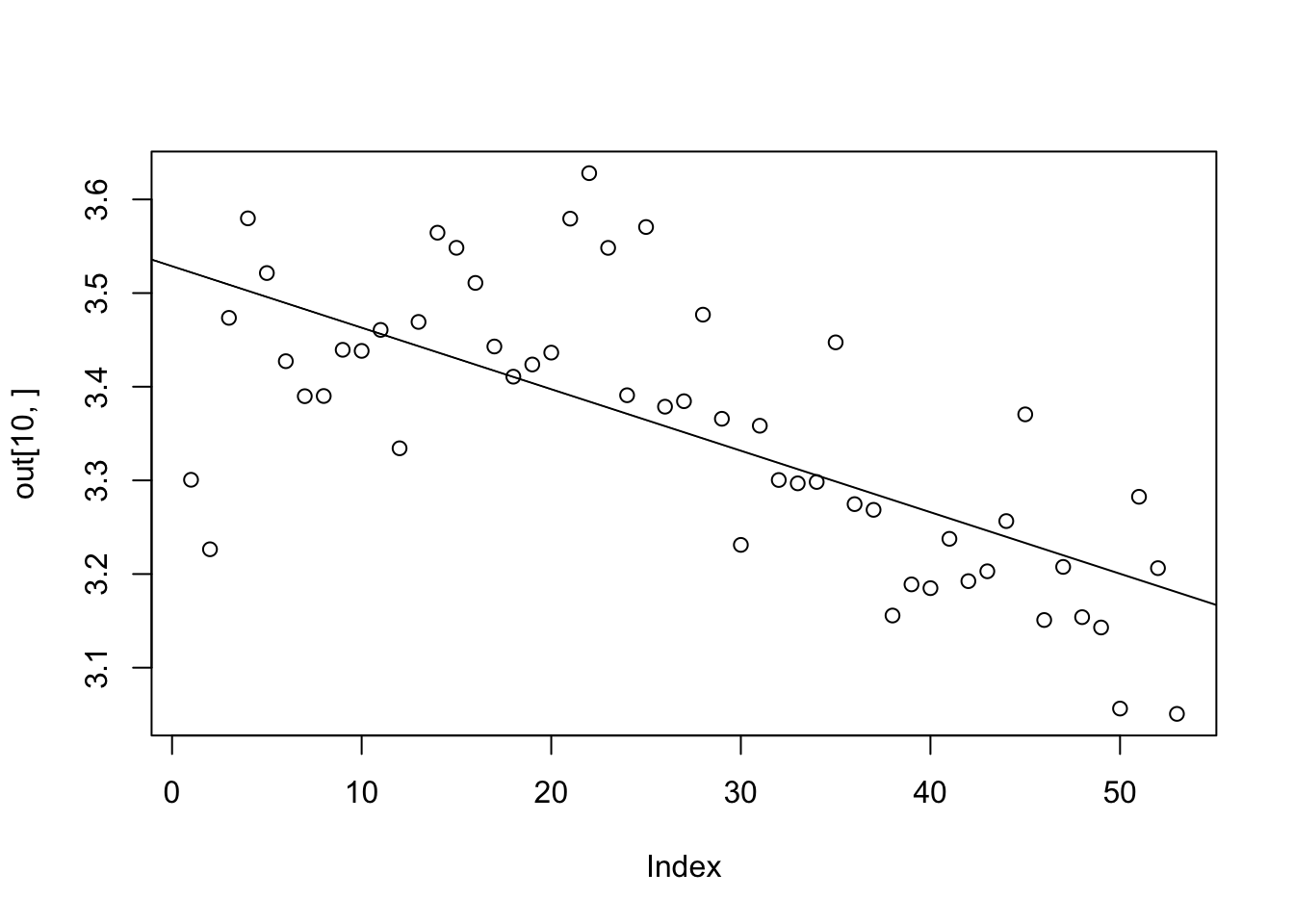

plot(out[10,])
lm(out[10,]~t) %>% summary %>%abline

Warning in abline(.): only using the first two of 8 regression coefficients

A.6.2 Using dplyr (tidyverse)

Base R

mtcars

                     mpg cyl  disp  hp drat    wt  qsec vs am gear carb
Mazda RX4           21.0   6 160.0 110 3.90 2.620 16.46  0  1    4    4
Mazda RX4 Wag       21.0   6 160.0 110 3.90 2.875 17.02  0  1    4    4
Datsun 710          22.8   4 108.0  93 3.85 2.320 18.61  1  1    4    1
Hornet 4 Drive      21.4   6 258.0 110 3.08 3.215 19.44  1  0    3    1
Hornet Sportabout   18.7   8 360.0 175 3.15 3.440 17.02  0  0    3    2
Valiant             18.1   6 225.0 105 2.76 3.460 20.22  1  0    3    1
Duster 360          14.3   8 360.0 245 3.21 3.570 15.84  0  0    3    4
Merc 240D           24.4   4 146.7  62 3.69 3.190 20.00  1  0    4    2
Merc 230            22.8   4 140.8  95 3.92 3.150 22.90  1  0    4    2
Merc 280            19.2   6 167.6 123 3.92 3.440 18.30  1  0    4    4
Merc 280C           17.8   6 167.6 123 3.92 3.440 18.90  1  0    4    4
Merc 450SE          16.4   8 275.8 180 3.07 4.070 17.40  0  0    3    3
Merc 450SL          17.3   8 275.8 180 3.07 3.730 17.60  0  0    3    3
Merc 450SLC         15.2   8 275.8 180 3.07 3.780 18.00  0  0    3    3
Cadillac Fleetwood  10.4   8 472.0 205 2.93 5.250 17.98  0  0    3    4
Lincoln Continental 10.4   8 460.0 215 3.00 5.424 17.82  0  0    3    4
Chrysler Imperial   14.7   8 440.0 230 3.23 5.345 17.42  0  0    3    4
Fiat 128            32.4   4  78.7  66 4.08 2.200 19.47  1  1    4    1
Honda Civic         30.4   4  75.7  52 4.93 1.615 18.52  1  1    4    2
Toyota Corolla      33.9   4  71.1  65 4.22 1.835 19.90  1  1    4    1
Toyota Corona       21.5   4 120.1  97 3.70 2.465 20.01  1  0    3    1
Dodge Challenger    15.5   8 318.0 150 2.76 3.520 16.87  0  0    3    2
AMC Javelin         15.2   8 304.0 150 3.15 3.435 17.30  0  0    3    2
Camaro Z28          13.3   8 350.0 245 3.73 3.840 15.41  0  0    3    4
Pontiac Firebird    19.2   8 400.0 175 3.08 3.845 17.05  0  0    3    2
Fiat X1-9           27.3   4  79.0  66 4.08 1.935 18.90  1  1    4    1
Porsche 914-2       26.0   4 120.3  91 4.43 2.140 16.70  0  1    5    2
Lotus Europa        30.4   4  95.1 113 3.77 1.513 16.90  1  1    5    2
Ford Pantera L      15.8   8 351.0 264 4.22 3.170 14.50  0  1    5    4
Ferrari Dino        19.7   6 145.0 175 3.62 2.770 15.50  0  1    5    6
Maserati Bora       15.0   8 301.0 335 3.54 3.570 14.60  0  1    5    8
Volvo 142E          21.4   4 121.0 109 4.11 2.780 18.60  1  1    4    2

# 1. Filter rows where mpg > 20
subset_data <- mtcars[mtcars$mpg > 20, ]

# 2. Select only mpg, cyl, hp columns
subset_data <- subset_data[, c("mpg", "cyl", "hp")]

# 3. Add new column kpg = mpg * 1.6
subset_data$kpg <- subset_data$mpg * 1.6

# 4. Order by descending mpg
subset_data <- subset_data[order(-subset_data$mpg), ]

subset_data <- subset(mtcars, mpg > 20, select = c(mpg, cyl, hp))
subset_data <- transform(subset_data, kpg = mpg * 1.6)
subset_data <- subset_data[order(-subset_data$mpg), ]

Now with tidyverse

library(dplyr)

mtcars |>
    filter(mpg > 20) |>
    dplyr::select(mpg, cyl, hp) |>
    mutate(kpg = mpg * 1.6) |>arrange(desc(mpg))

                mpg cyl  hp   kpg
Toyota Corolla 33.9   4  65 54.24
Fiat 128       32.4   4  66 51.84
Honda Civic    30.4   4  52 48.64
Lotus Europa   30.4   4 113 48.64
Fiat X1-9      27.3   4  66 43.68
Porsche 914-2  26.0   4  91 41.60
Merc 240D      24.4   4  62 39.04
Datsun 710     22.8   4  93 36.48
Merc 230       22.8   4  95 36.48
Toyota Corona  21.5   4  97 34.40
Hornet 4 Drive 21.4   6 110 34.24
Volvo 142E     21.4   4 109 34.24
Mazda RX4      21.0   6 110 33.60
Mazda RX4 Wag  21.0   6 110 33.60

Much better with

pak::pak("hadley/genzplyr")

✔ Updated metadata database: 8.00 MB in 10 files.

ℹ Updating metadata database

✔ Updating metadata database ... done

ℹ No downloads are needed

✔ 1 pkg + 15 deps: kept 10 [50.7s]

library(genzplyr)

genzplyr loaded fr fr 💅
Your data wrangling is about to be bussin no cap

mtcars |>
  yeet(mpg > 20) |>
  vibe_check(mpg, cyl, hp) |>
  glow_up(kpg = mpg * 1.6) |>
  slay(desc(mpg))

                mpg cyl  hp   kpg
Toyota Corolla 33.9   4  65 54.24
Fiat 128       32.4   4  66 51.84
Honda Civic    30.4   4  52 48.64
Lotus Europa   30.4   4 113 48.64
Fiat X1-9      27.3   4  66 43.68
Porsche 914-2  26.0   4  91 41.60
Merc 240D      24.4   4  62 39.04
Datsun 710     22.8   4  93 36.48
Merc 230       22.8   4  95 36.48
Toyota Corona  21.5   4  97 34.40
Hornet 4 Drive 21.4   6 110 34.24
Volvo 142E     21.4   4 109 34.24
Mazda RX4      21.0   6 110 33.60
Mazda RX4 Wag  21.0   6 110 33.60

# Complete analysis that's absolutely bussin
mtcars |>
  yeet(hp > 100) |>                    # Yeet the weak cars
  vibe_check(mpg, cyl, hp, wt) |>      # Vibe check our columns
  glow_up(                              # Glow up the data
    hp_per_ton = hp / (wt / 2),
    efficiency = mpg / (hp / 100)
  ) |>
  squad_up(cyl) |>                     # Squad up by cylinders
  no_cap(                               # Get the real stats
    avg_hp = mean(hp),
    avg_mpg = mean(mpg),
    avg_efficiency = mean(efficiency),
    squad_size = n()
  ) |>
  disband() |>                         # Disband the squads
  slay(desc(avg_efficiency)) |>        # Sort by slay factor
  send_it(10)

# A tibble: 3 × 5
    cyl avg_hp avg_mpg avg_efficiency squad_size
  <dbl>  <dbl>   <dbl>          <dbl>      <int>
1     4   111     25.9          23.3           2
2     6   122.    19.7          16.6           7
3     8   209.    15.1           7.67         14

A.6.3 Introduction to gpplot2

ggplot2 is based on ideas from the book “A grammar of graphics” by Leland Wilkinson and developed by Hadley Wickham, which also developed tidyverse.

library(ggplot2)

cars

   speed dist
1      4    2
2      4   10
3      7    4
4      7   22
5      8   16
6      9   10
7     10   18
8     10   26
9     10   34
10    11   17
11    11   28
12    12   14
13    12   20
14    12   24
15    12   28
16    13   26
17    13   34
18    13   34
19    13   46
20    14   26
21    14   36
22    14   60
23    14   80
24    15   20
25    15   26
26    15   54
27    16   32
28    16   40
29    17   32
30    17   40
31    17   50
32    18   42
33    18   56
34    18   76
35    18   84
36    19   36
37    19   46
38    19   68
39    20   32
40    20   48
41    20   52
42    20   56
43    20   64
44    22   66
45    23   54
46    24   70
47    24   92
48    24   93
49    24  120
50    25   85

plot(cars$speed,cars$dist)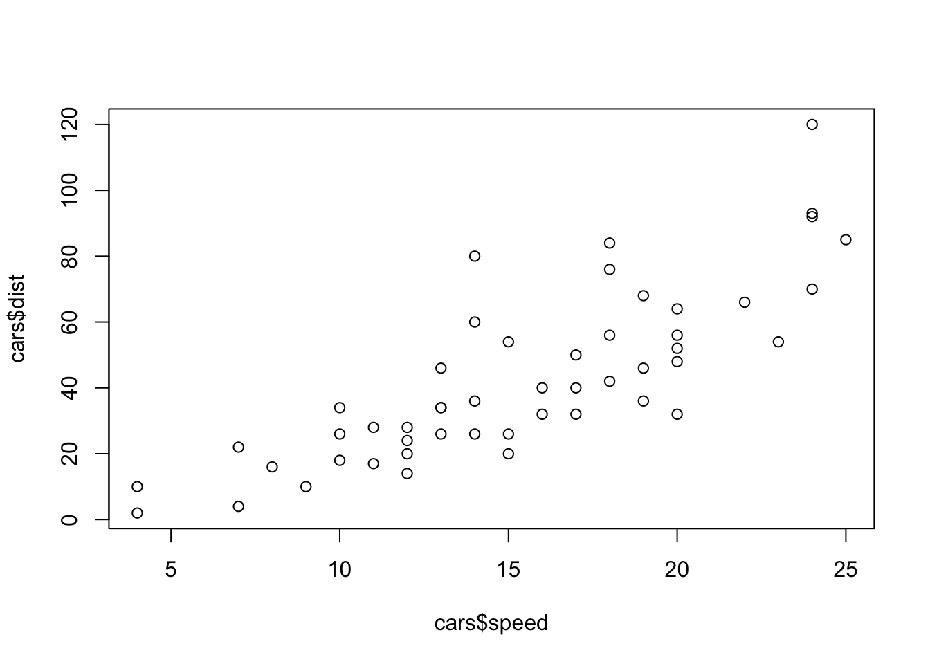

ggplot(data=cars, mapping=aes(x=speed,y=dist)) + geom_point(colour="red")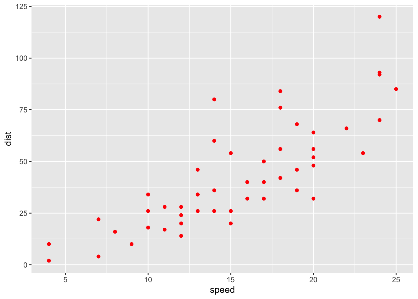

myplot <-  ggplot(cars, aes(speed,dist))+
  geom_point()+geom_line()
myplot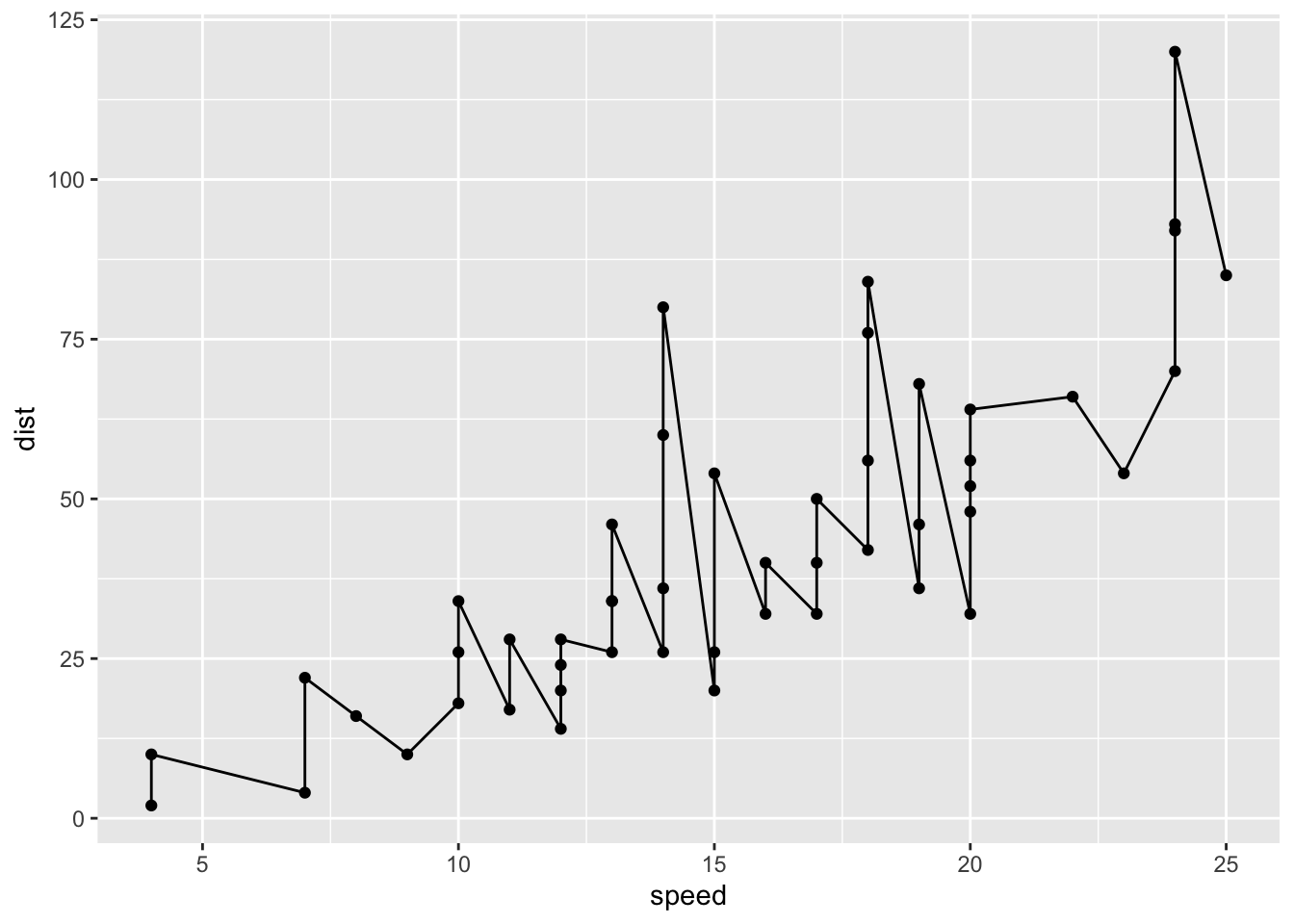

data(cars)
myplot <-  ggplot(cars, aes(speed,dist))+
  geom_point()+geom_smooth(method="lm")
myplot

`geom_smooth()` using formula = 'y ~ x'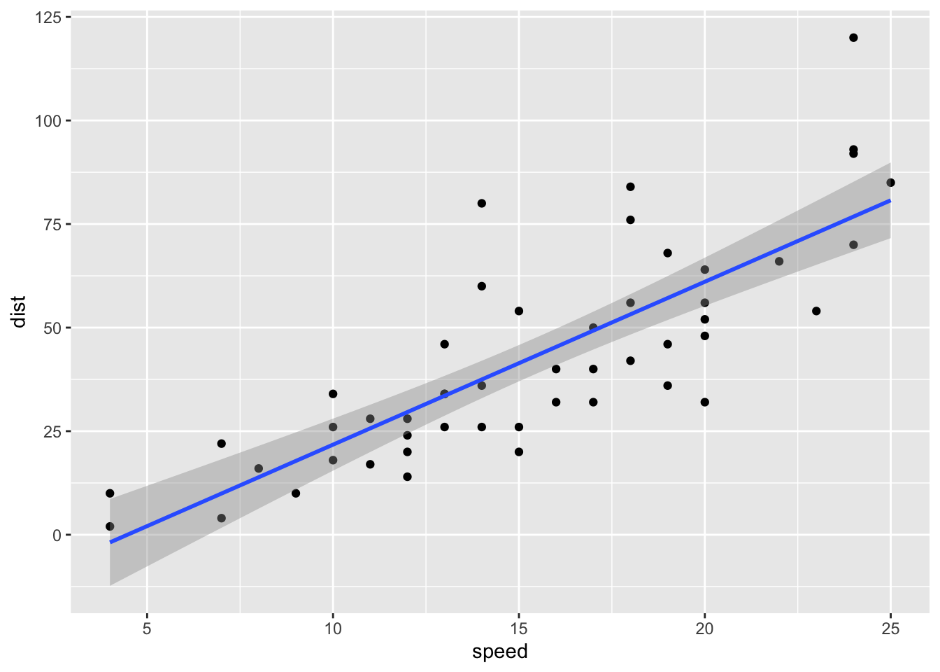

data(cars)
myplot <-  ggplot(cars, aes(speed,dist))+
  geom_point()+geom_smooth(method="lm")+scale_x_log10()+scale_y_log10()
myplot

`geom_smooth()` using formula = 'y ~ x'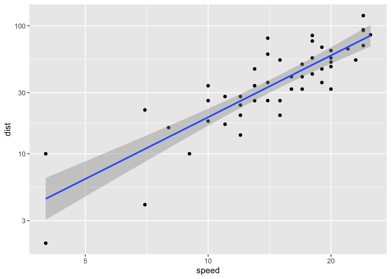

With tidyplot

library(tidyplots)
cars |>  tidyplot(x=speed,y=dist) |>
  add_data_points_beeswarm() |>
  add_curve_fit(method="lm")

`geom_smooth()` using formula = 'y ~ x'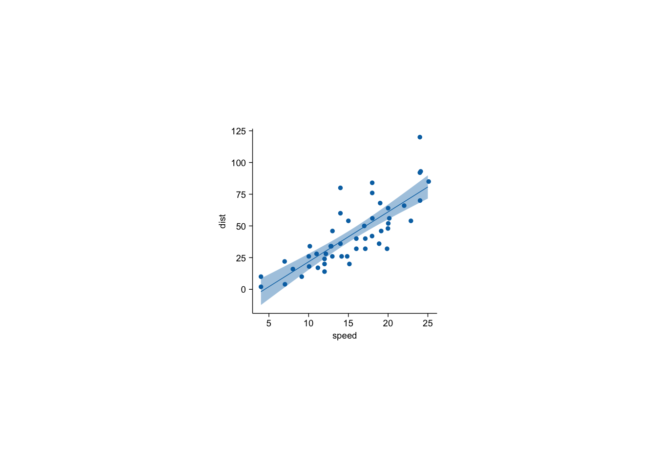

cars |>  tidyplot(x=speed,y=dist) |>
  add_data_points_beeswarm() |>
  add_curve_fit()

`geom_smooth()` using formula = 'y ~ x'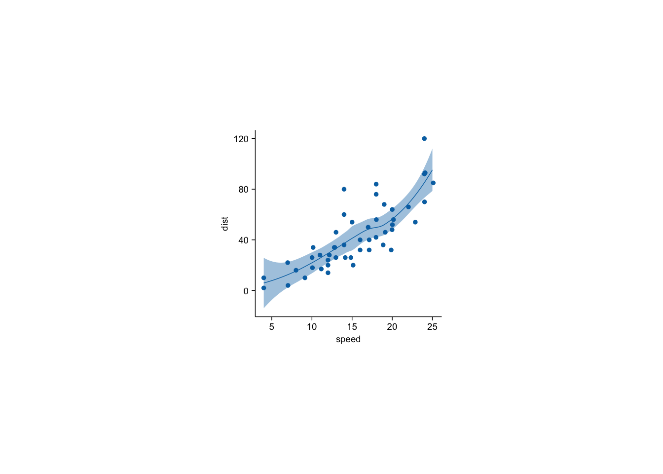

With the florida data

#ggplot
mat=cbind(t,out[10,])
colnames(mat)<-c("time","shannon")
mat<-as.data.frame(mat)

myplot <-  ggplot(mat, aes(time,shannon))+
  geom_point()
myplot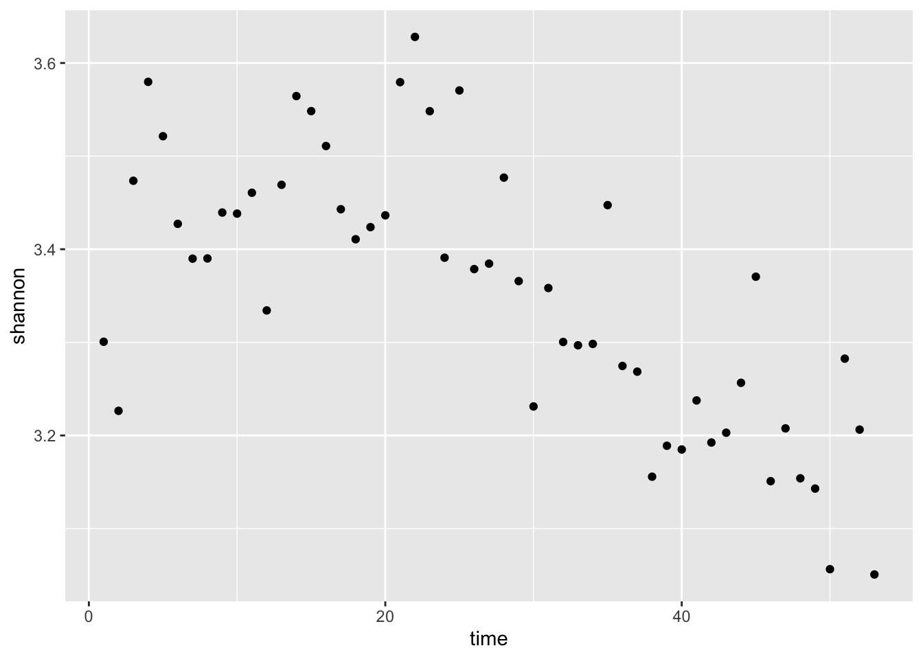

myplot <-  ggplot(mat, aes(time,shannon))+
  geom_line()
myplot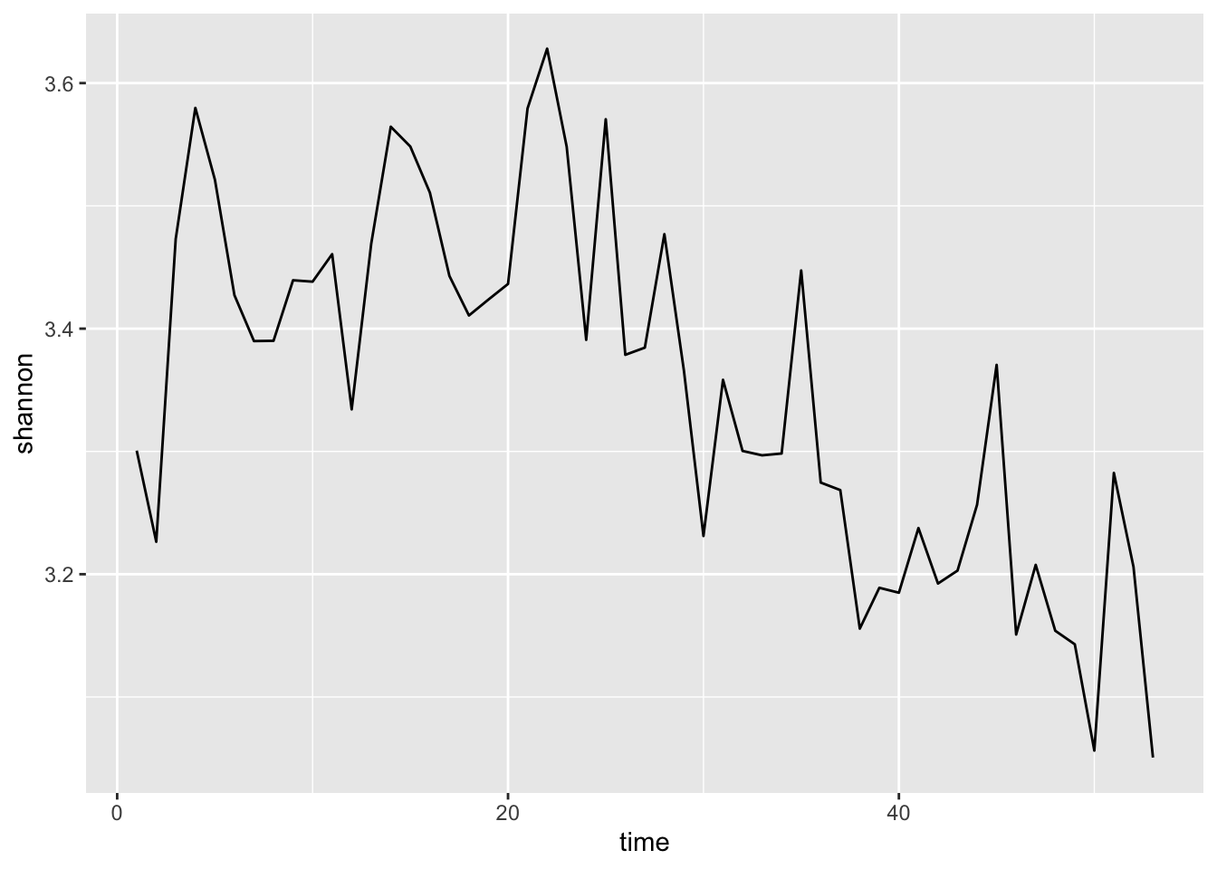

A.7 Working with biodiversity data: GBIF, EBV Portal

Authors: Corey Callaghan, Luise Quoss, Isabel Rosa.

First we load the library rgbif

library(rgbif)
library(tidyverse)

Now we will download observations of a species. Let’s download observations of the common toad Bufo bufo.

matbufobufo<-occ_search(scientificName="Bufo bufo", limit=500, hasCoordinate = TRUE, hasGeospatialIssue = FALSE)

Error in occ_search(scientificName = "Bufo bufo", limit = 500, hasCoordinate = TRUE, : could not find function "occ_search"

Let’s examine the object matbufobufo

class(matbufobufo)

Error: object 'matbufobufo' not found

matbufobufo

Error: object 'matbufobufo' not found

It is a special object of class gbif which allows for the metadata and the actual data to all be included, as well as taxonomic hierarchy data, and media metadata. We won’t worry too much about the details of this object now.

Let’s download data about octupusses. They are in the order “Octopoda”. First we need to find the GBIF search key for Octopoda.

a<-name_suggest(q="Octopoda",rank="Order")

Error in name_suggest(q = "Octopoda", rank = "Order"): could not find function "name_suggest"

key<-a$data$key

Error: object 'a' not found

We will only download 2000 observations to keep it simple for now. If you were doing this for real, you would download all data.

octopusses<-occ_search(orderKey=key,limit=2000, hasCoordinate = TRUE, hasGeospatialIssue = FALSE)

Error in occ_search(orderKey = key, limit = 2000, hasCoordinate = TRUE, : could not find function "occ_search"

Show the result

octmat<-octopusses$data

Error: object 'octopusses' not found

head(octmat)

Error: object 'octmat' not found

Count the number of observations per species using tidyverse and pipes

octmat %>% 
  group_by(scientificName) %>% 
  summarise(sample_size=n()) %>%
  arrange(desc(sample_size)) %>% 
  mutate(sample_size_log=log(sample_size,2)) %>% 
  ggplot(aes(x = sample_size_log)) + geom_histogram()

Error: object 'octmat' not found

Plot the records on an interactive map. First load the leaflet package.

library(leaflet)
leaflet(data=octmat) %>% addTiles() %>%
  addCircleMarkers(lat= ~decimalLatitude, lng = ~decimalLongitude,popup=~scientificName)